Many users don’t know how to check whether a row is hidden or visible in Google Sheets. The question of how to highlight the row above the hidden row comes next.
Without knowing this (finding hidden row), it’s impossible to write formulas that only include visible rows or hidden rows in a range.
There are two tips in this post – a formula tip and a conditional formatting tip. Let’s start with the first one.
How to Test Whether a Row Is Hidden or Visible in Google Sheets
To test a hidden row, you can consider any non-blank cell in that row.
If a row is entirely blank then you can’t check whether that row is hidden or visible in Google Sheets. Also, the cell that you consider for the hidden row test must not contain any SUBTOTAL formula.
What about an Example to Check a Hidden Row in Google Sheets?
Here is one! I will explain the scenario/problem with an easy to understand example.
Assume, you want to check whether cell A5 (row # 5) is hidden or not in a sheet. Then what you may want to do is to insert the below SUBTOTAL formula in any other row.
=subtotal(103,A5)
As I have mentioned at the beginning, the cell A5 must contain any characters and shouldn’t contain any SUBTOTAL formula.
If row # 5 is hidden, the result of the above formula will be zero. To get a custom message like “hidden” or “not hidden”, use the IF function (if this, then that) with SUBTOTAL.
=if(subtotal(103,A5)=0,"hidden","not hidden")
This way you can check whether a row is hidden or visible in Google Sheets. Here is the second tip.
How to Highlight the Rows above Hidden Rows in Google Sheets
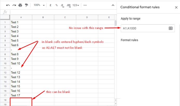
This will only work if you have a column without blank cells within the data range. If there are blanks, insert a hyphen/dash symbol or 0 in those blank cells.
For example, my data range is A1:A17. I can include the range A1:A1000 or A1:Z1000 to apply the conditional formatting. But A1:A17 must not be blank. I hope, the below image will speak better.
For those who want to keep blank cells, there is one more option!
Use an extra blank column (we can call it a helper column). In the very first cell in that column, key this SEQUENCE formula in.
=sequence(rows(A:A),1)
Then hide the column. Use that column in formulas instead of the ‘real’ range.
I mean, since there are no blank cells, I am using column A in my formulas below. Assume there are blank cells in column A.
Then, if the above sequence formula is in cell D1, that means column D is the helper column, use column D in your formulas instead of column A. Let’s begin.
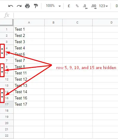
How to know, without using a formula, whether there are rows hidden in a sheet?
Looking at the unhide button (black up ▲ and down ▼ pointing triangles) or checking the row numbers, right?
If you want, you can highlight the row just above the hidden row to easily find/identify the hidden rows.
First, I will show you how the output will look like. If you seem interested in such conditional formatting, then only proceed further.
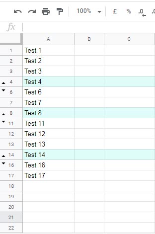
Since the rows 5, 9, 10, and 15 are hidden, the rows just above these rows (i.e. rows 4, 8, and 14) got highlighted.
By highlighting so, without checking the row numbers or the black up and down pointing triangles, you can identify the rows (location) hidden on your entire sheet.
Custom Formulas Rules for Highlighting
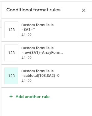
To highlight the rows above hidden rows as above, we can use three custom formulas in the Conditional Formatting in Google Sheets. They are as follows.
Rule (Formula) # 1:
Fill color is ‘None’.
=$A1=""Rule (Formula) # 2:
Fill color is ‘None’.
=row($A1)=ArrayFormula(MATCH(2,1/($A:$A<>" "),1))Rule (Formula) # 3:
Use your choice of color other than none/white.
=subtotal(103,$A2)=0In the Format menu Conditional formatting (Format > Conditional formatting > Format rules > Custom formula is), insert the above formulas in the same formula order.
Format Rules Formulas – Explanation
Rule # 1 is for removing any highlighting in blank rows in the range.
For example, see my data. It’s in A1:A17. I am applying my rules to the whole sheet (A1:Z1000). So the rows 18 to below are blank. This rule will remove any highlighting below row # 17.
The purpose of Rule # 2 is to find the last non-blank cell in column A (it’s row # 17) and remove any highlighting in that row. Why this rule is required? Rule # 3 is the answer.
Rule # 3 checks whether a row is hidden and highlight the row above the hidden row.
Normally conditional format rule will apply to the row referenced in the formula rule. We want to skip the highlighting to one row up. I mean test one cell and highlight the cell above it.
Here is the trick. I have selected the range A1:Z1000 (apply to range) in conditional formatting. Rule # 3 formula tests whether a cell (row) is hidden or not from row # 2 to downwards.
Since ‘apply to range’ (A1:Z1000) starts from A1 (row # 1 to downwards) and formula rule starts from A2 (row # 2 to downwards), the highlighting related to row # 2 will apply to # 1. The same will repeat to the rows down.
This makes one issue when we reach the last non-blank row which is row # 17. What’s that issue?
Rule # 3 formula will return 0 in a non-blank cell other than a hidden row. A18 is blank so the formula will return 0 and will ‘wrongly’ consider row # 18 as blank and eventually highlight row # 17.
I have used the second rule to remove this unwanted highlighting in the last non-blank row.
Google Sheets Popular Functions in Hidden | Visible Rows
- Google Sheets Query Hidden Row Handling with Virtual Helper Column.
- SUMIF Excluding Hidden Rows in Google Sheets Without Helper Column.
- How to Omit Hidden or Filtered out Values in Sum Google Doc Spreadsheet.
- Vlookup Skips Hidden Rows in Google Sheets – Formula Example.
- Find the Average of Visible Rows in Google Sheets.
- Count Unique Values in Visible Rows in Google Sheets.
- Highlight Visible Duplicates in Google Sheets.
- IMPORTRANGE to Import Visible Rows in Google Sheets.
Crawlan.com is a great resource for more Google Sheets tips and tricks.


