Combine Data Dynamically in Multiple Tabs Vertically in Google Sheets

In this Google Sheets tutorial, I’m going to share with you a game-changing technique that will allow you to combine data dynamically from multiple sheet tabs. Are you tired of copying and pasting data or specifying each range individually? Well, fret no more because I have the perfect solution for you!

The Challenge of Organizing Data in Multiple Tabs

Google Sheets and similar apps provide the convenience of organizing data in sheet tabs within a workbook. However, when it comes to creating a summary of data from multiple tabs, things can get a bit tricky. Let’s say you have monthly data organized in different tabs in Google Sheets. You might find yourself copying and pasting this data into a master sheet, or worse, manually specifying each range within a formula.

Introducing the COPY_TO_MASTER_SHEET Function

To overcome the hassle of copy-pasting or individually specifying data ranges, I present to you the COPY_TO_MASTER_SHEET function. This custom-named function will revolutionize the way you combine data vertically from multiple sheet tabs in Google Sheets.

Features of the Formula for Dynamically Combining Sheet Tabs Vertically

The COPY_TO_MASTER_SHEET formula, also known as the named function, comes with a range of powerful features that will streamline your data organization process:

• Vertical and Sequential Appending: The formula appends data vertically and in sequence, creating a larger array. This means that the data from the second sheet will be positioned right beneath the first sheet, the data from the third sheet beneath the second sheet, and so on.

• Retention of Data Types: Unlike other methods that involve using the SPLIT function, neither the COPY_TO_MASTER_SHEET function nor the formula uses it, ensuring that the data types in the result are preserved.

• Recommendation for Closed Data Ranges: To avoid potential issues with blank rows, it is recommended to use closed data ranges in the formula. For example, instead of using A1:C, use A1:C1000. However, if you prefer an open range, you can wrap the named function or formula with QUERY or FILTER to filter out any blank rows.

Prerequisites

Assuming you want to dynamically combine data from Sheet1, Sheet2, and Sheet3 into a fourth sheet named Master, here’s what you need to do. In the Master sheet, you should have a list of all tab names in column A. You can manually enter these names or use a Google Apps Script, which you can obtain by following these steps:

1. Go to the “Extensions” menu in your Google Sheets and select “Apps Script.”
2. Delete the default text and copy-paste the Apps Script from the provided source.
3. Save the project by selecting the floppy icon.

Alternatively, you can create a copy of my sample sheet that I’ve provided a few paragraphs below.

To get all tab names in cell A1 on your Master sheet, use the following formula:

=sheetnames()

When using the COPY_TO_MASTER_SHEET function or formula to combine data from the “Sheet1,” “Sheet2,” and “Sheet3” tabs into the “Master” sheet, make sure to specify only A2:A and not A1:A. This is because A1 will contain the name “Master,” which you don’t want to include in the combination.

Combine Data Dynamically in Multiple Tabs Vertically: Formula

Let’s put the formula into action! Imagine you have data in Sheet1, Sheet2, and Sheet3, and you want to merge it vertically into the Master sheet. Here’s how you can achieve that:

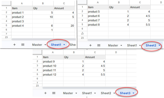
The above image shows the expected output after dynamically merging the data from sheets 1 to 3 vertically.

To achieve this, you can use the following formula:

=REDUCE( TOCOL(, 1), TOCOL(A2:A, 1), LAMBDA(a, v, IFERROR(VSTACK(a, INDIRECT(v&"!"&"A2:C5")))) )

Let’s break down the formula:

• A2:A is the list of tab names.
• “A2:C5” is the range in each sheet to merge vertically.

If you prefer using open ranges, for example, “A2:C” instead of “A2:C5”, make sure to wrap the formula with QUERY, like this:

=QUERY(..., "SELECT * WHERE Col1 IS NOT NULL", 0)

Now, let me explain how the formula dynamically combines multiple sheet tabs vertically in Google Sheets.

Formula Breakdown

The formula utilizes the REDUCE function to seamlessly combine multiple sheet tabs vertically. Here’s how the syntax looks:

REDUCE(initial_value, array_or_range, lambda)

In the formula:

• initial_value: TOCOL(, 1) – The TOCOL function returns an empty cell when specified as TOCOL(, 0). By changing 0 to 1, we eliminate that empty cell, fulfilling the initial_value requirement for REDUCE. Essentially, it returns nothing.
• array_or_range: TOCOL(A2:A, 1) – This part returns the list of sheet names, removing any empty cells.

The lambda function part of the formula includes:

• a: Name of the accumulator.
• v: Each value (sheet name) from array_or_range.

The REDUCE function iterates over each sheet name in the array_or_range using the function INDIRECT(v&"!A2:C5"). In each iteration, v represents Sheet1, Sheet2, and Sheet3.

The result at each step is stored in the accumulator, which is then vertically stacked using VSTACK as VSTACK(a, ...). This summarizes the REDUCE logic behind dynamically combining multiple sheets vertically.

Combine Data Dynamically in Multiple Tabs Vertically: Named Function

If you find it more convenient to work with custom-named functions, don’t worry—I’ve got you covered! The above formula is already custom-named function-ready.

Simply copy-paste it into the formula definition part of your Google Sheets by navigating to the Data menu, selecting Named functions, and adding a new function. Replace the cell range references with names and add those names within argument placeholders.

Here’s what the syntax of the named function looks like:

COPY_TO_MASTER_SHEET(list, array)

And here are the arguments:

• list: The cell or cell range that contains the tab list to combine.
• array: The range of data to combine, specified within double quotation marks.

For example, you can replace the earlier formula in Master!B2 with the COPY_TO_MASTER_SHEET named function like this:

=COPY_TO_MASTER_SHEET(A2:A,"A2:C5")

If you want to combine multiple sheets dynamically with open ranges, use the following formula that includes QUERY:

=QUERY(COPY_TO_MASTER_SHEET(A2:A,"A2:C"), "SELECT * WHERE Col1 IS NOT NULL", 0)

Thanks to the named function, anyone can quickly combine data from multiple sheet tabs into a master sheet tab in Google Sheets.

How to Copy the COPY_TO_MASTER_SHEET Named Function

Let me walk you through the steps of copying the named function:

1. Import the named function into the sheet where you want to use it.
2. Make a copy of my sample sheet provided above.
3. Go to File > Settings and under “Locale,” select the same country as the sheet in which you want to use my function.
4. Open the sheet in which you want to use the COPY_TO_MASTER_SHEET function.
5. Go to the Data menu in that sheet, select Named functions > Import function.
6. Select the copied sheet (you can search by sheet name) and click Insert. Follow the onscreen instructions.

You will find the code to import, making it easy for you to start using the COPY_TO_MASTER_SHEET named function.

Resources

If you’re hungry for more Google Sheets knowledge, here are some additional resources that you might find useful:

1. Consolidate Data from Multiple Sheets Using a Formula in Google Sheets
2. Consolidate Only the Last Row in Multiple Sheets in Google Sheets
3. How to Combine Multiple Sheets in Importrange and Control Via Drop-Down
4. Dynamically Combine Multiple Sheets Horizontally in Google Sheets
5. SUMIF Across Multiple Sheets in Google Sheets
6. Vlookup Across Multiple Sheets in Google Sheets
7. How to Include Future Sheets in Formulas in Google Sheets

I hope this tutorial has provided you with valuable insights into combining data dynamically in multiple tabs vertically in Google Sheets. Until next time, happy spreadsheeting!

Crawlan.com