Compare Two Google Sheets Cell by Cell and Highlight

Have you ever wanted to compare two Google Sheets and easily identify the differences or matches between them? Look no further! In this article, I’ll show you how to perform a cell-by-cell comparison of two Google Sheets and highlight the variations. Whether you have two sheets in the same file or in different files, my formula will work seamlessly for you.

Two Tabs in the Same Google Sheets File

Let’s start by comparing two tabs within the same Google Sheets file and highlighting any differences.

To begin, imagine you have two tabs named “Sheet1” and “Sheet2” within your Google Sheets file. In both sheets, let’s say you have limited the number of rows to 10 and columns to 5 to speed up the highlighting process.

Now, select the range of cells that you want to compare. It’s recommended to choose only the ranges with data to improve the performance of your sheet.

Here’s the fun part – the cell-by-cell comparison! Each cell in Sheet1 will be compared to the corresponding cell in Sheet2. If the values don’t match, my custom formula will highlight the corresponding cell in Sheet1. But don’t worry, you can also choose to highlight Sheet2 if you’d like.

Let’s take a look at the contents of the two Sheet Tabs:

Table 1 in Sheet1:

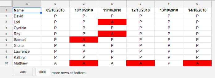
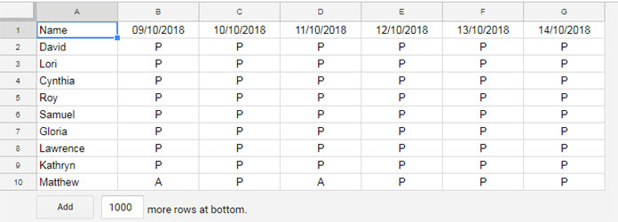
Table 1 in Sheet2:

To highlight the differences, you can use the following formula as a custom rule in your conditional formatting:

=A1<>(Indirect("Sheet2!"&Address(Row(),Column(),)))

Here’s how you can apply this conditional formatting formula to compare and highlight differences in your sheet:

1. Click on the “Format” menu.
2. Select “Conditional format” from the drop-down menu.
3. Apply the above formula in the custom formula field within the conditional format window.

Voila! The differences between the two sheets will now be highlighted in Sheet1.

But what if you want to highlight the matches instead? Don’t worry, I’ve got you covered.

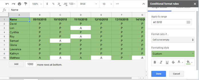
To highlight the matches, simply use the same custom formula from earlier. However, instead of using the color red to highlight the matches, change it to white. Yes, you heard me right! White is your conditional formatting rule #1.

Next, add a new conditional formatting rule and choose the color red or any other color of your choice. But this time, select “Cell is not empty” under the “Format cells if…” option.

For visual reference, please see the following image:

If you want the highlighting to appear in both tabs, you can use the following formula in Sheet2:

=A1<>(Indirect("Sheet1!"&Address(Row(),Column(),)))

By changing “Sheet2” to “Sheet1” in the formula above, you’ll achieve the highlighting in both tabs.

That covers the cell-by-cell comparison of two tabs within the same Google Sheets file for differences or matches.

One Tab Each in Two Different Google Sheets Files

Now let’s explore how to compare two different Google Spreadsheet files cell by cell.

Before diving into this section, please ensure that you have properly tested and understood the formulas explained above for comparing two sheets within the same file.

Assuming you’ve grasped that concept, let’s move on.

In this scenario, let’s say we have two different Google Sheets files: “attendance1” and “attendance2”. The sheet names within these files are “A1” and “B2”, respectively.

To apply conditional formatting between these two Google Spreadsheets files, you’ll first need to link them together. Here’s how:

1. Insert a new sheet tab in the “attendance1” file and name it “A2”.
2. In cell A1 of this new sheet tab, use the following formula:

   =IMPORTRANGE("URL","B2!A1:G10")

   Replace “URL” in the formula with the URL of the “attendance2” file, which you can copy from the address bar of your browser.

If the formula returns a “#REF!” error, click on it and allow access.

Finally, apply the same conditional formatting formula from earlier to the “A1” sheet in the “attendance1” file. Choose the color that you want to highlight the differences.

To compare cell by cell and highlight matches, refer to the example mentioned under the subsection titled “Compare Two Google Sheets Cell by Cell and Highlight The Matches”.

That’s it! You’ve now learned how to compare two Google Sheets cell by cell and highlight the differences or matches, both within the same file and between different files.

For additional resources, check out these related articles:

1. How to Conditional Format Duplicates Across Sheet Tabs in Google Sheets
2. Role of Indirect Function in Conditional Formatting in Google Sheets

For more exciting tips and tricks, visit Crawlan.com.