Are you struggling to use Countifs with multiple criteria in the same range in Google Sheets? If so, you’ve come to the right place. In this tutorial, I’ll show you how to efficiently handle and count multiple criteria using Countifs in Google Sheets.
Countifs OR Criteria Within Curly Brackets in Sheets and Excel
To use multiple criteria in the same column range in COUNTIFS, we can make use of Curly Braces. This technique applies to both Excel and Google Sheets. Here’s an example formula for multiple criteria in the same column range in Countifs:
=SUM(COUNTIFS(A:A,{"APPLE","ORANGE","POMEGRANATES"}))In Google Sheets, you must also use ArrayFormula with Curly Braces to achieve the same effect. Here’s the modified formula for Google Sheets:
=ArrayFormula(SUM(COUNTIFS(A:A,{"APPLE","ORANGE","POMEGRANATES"})))Countifs with Multiple Criteria in the Same Range in Excel
Let’s dive into Excel and see how we can use Countifs with multiple criteria in the same range. For this example, we’ll consider a two-column data set.
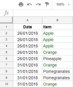
Suppose we want to count the number of occurrences of different fruit items on a particular date. In this case, we’ll use today’s date (31/01/2018) as our reference. To count the items “Apple”, “Orange”, and “Pomegranates” that appear on this date, we can use the following formula:
=SUM(COUNTIFS(A:A,TODAY(),B:B,{"APPLE","ORANGE","POMEGRANATES"}))Countifs with Multiple Criteria in the Same Range in Google Sheets
Contrary to popular belief, you can use Countifs with multiple criteria in the same range in Google Sheets. Many users mistakenly assume that this is not possible or recommended in Google Sheets. However, we can achieve the desired result by wrapping the Excel formula with the ArrayFormula function in Google Sheets. Here’s the modified formula:
=ArrayFormula(SUM(COUNTIFS(A:A,TODAY(),B:B,{"APPLE","ORANGE","POMEGRANATES"})))Countif + If Alternative to Countifs in Google Sheets
In Google Sheets, we can intelligently replace the Countifs formula with an IF+Countif combination. Here’s the formula:
=ARRAYFORMULA(SUM(COUNTIF(IF(A1:A=TODAY(),B1:B),{"APPLE","ORANGE","POMEGRANATES"})))The use of the IF function in this formula allows us to return all values in column B if the corresponding values in column A match today’s date. We then use a Countif formula to count the occurrences of the specified items in the resulting range.
Conclusion
With this tutorial, I hope I’ve shed some light on the usage of Countifs with multiple criteria in the same range in Google Sheets. Don’t let the misconception discourage you – it is indeed possible and recommended. By following the techniques explained here, you can efficiently count and handle multiple criteria in your Google Sheets. Stay tuned for more advanced Google Sheets tutorials on Crawlan.com.
Additional Resources:
- COUNTIFS in a Time Range in Google Sheets [Date and Time Column]
- Google Sheets: Countifs with Not Equal to in Infinite Ranges
- How to Perform a Case Sensitive COUNTIF in Google Sheets
- Countif in an Array in Google Sheets Using Vlookup and Query Combo
- How to Use COUNTIF with UNIQUE in Google Sheets
- COUNTIF to Count by Month in a Date Range in Google Sheets


