Sometimes, we find ourselves in a situation where we need to extract search keys and use Vlookup in Google Sheets. This tutorial will teach you how to do just that. But before we dive in, let me draw your attention to a related scenario involving vertical lookup (Vlookup)!
What’s the scenario? Well, if a search key is part of a text (substring) in the lookup table’s first column within the range, we can use wildcard characters with the search key. You can learn more about using wildcard characters in Google Sheets functions here.
Here’s the Vlookup syntax for reference: VLOOKUP(search_key, range, index, [is_sorted]). I’ve also explained this in more detail in my post on Partial Match in Vlookup in Google Sheets.
Now, let’s move on to our main topic – how to extract search keys and use Vlookup in a table in Google Sheets.
When Should One Extract Search Keys and Vlookup in Google Sheets?
To better understand this, let’s consider an example with the range A1:B4:
| First Name | Advance |
|---|---|
| Martha | 5400 |
| Diana | 5000 |
| Harold | 0 |
In this example, let’s say our search key for vertical lookup is “Diana Reed”. If we use the following Vlookup formula, it would return #N/A: =vlookup("Diana Reed",A1:B4,2,0). Why? Because the search key is not available in the first column of the lookup table.
In simpler terms, we have a first name and last name together as the search key to Vlookup a table that only contains first names. To perform this type of vertical lookup, we need to extract the search key, which is the first name, and then do the Vlookup.
To illustrate this, let’s take a closer look at the following example:

In this example, the full name “Diana Reed” is the search key in cell D2. We need to systematically extract the search key (first name) only from this cell and use it in the Vlookup formula in cell E2.
To extract the search key, i.e. the first name, we can use the REGEXEXTRACT function along with the SORTN formula. Here’s the formula: =SORTN(REGEXEXTRACT(D2,A2:A4)). This formula will match the first names in column A with the name in cell D2 and extract the matching string.
Now, let’s use this extracted search key as the search key in Vlookup with the following formula: =vlookup(SORTN(REGEXEXTRACT(D2,A2:A4)),A1:B4,2,0).
That’s it! You can now use this method to extract search keys and perform Vlookup in Google Sheets.
How Do We Extract Multiple Search Keys and Vlookup Them in Google Sheets?
There are times when we need to use multiple search keys in Vlookup. This means we want to return a Vlookup array result. Let’s consider another example:
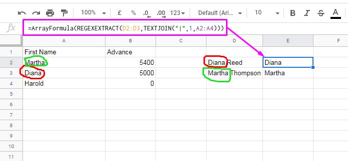
In this example, we have two search keys to extract – the first and last names in cells D2 and D3. To extract multiple search keys for Vlookup, we can use the REGEXEXTRACT function along with the TEXTJOIN formula. Here’s the formula: =ArrayFormula(REGEXEXTRACT(D2:D3,TEXTJOIN("|",1,A2:A4))).
Now, let’s use this formula as the search keys in Vlookup with the following formula: =ArrayFormula(vlookup(REGEXEXTRACT(D2:D3,TEXTJOIN("|",1,A2:A4)),A2:B4,2,0)). This Vlookup formula will return 5000 in cell E2 and 5400 in cell E3.
Conclusion
In real-life scenarios, we can use the above Vlookup techniques to assign values to a table. For example, if you have a column with campaign names in Sheet1!A1:A, and you want to assign campaign types from a table in Sheet2!A1:B, you can use the following formula: =ArrayFormula(IFNA(vlookup(REGEXEXTRACT(A1:A,TEXTJOIN("|",1,Sheet2!A2:A4)),Sheet2!A2:B4,2,0))).
That’s all there is to extracting search keys and performing Vlookup in Google Sheets. I hope you found this tutorial helpful. If you have any questions, feel free to reach out at Crawlan.com.
Enjoy exploring the world of Google Sheets!


