Are you using Vlookup in Google Sheets? If so, you may not be aware of a powerful technique that can enhance its functionality. By combining Filter with Vlookup result columns, you can unlock a whole new world of possibilities. In this tutorial, we will explore the benefits and provide you with practical examples to help you make the most out of this feature.
Introduction: Unleashing the Power of Vlookup in Google Sheets
As a Google Sheets expert, I have always believed that Vlookup in Google Sheets surpasses its Excel counterpart in terms of versatility and flexibility. With Google Sheets, you have the freedom to customize Vlookup to meet your unique requirements. There are three key reasons why Google Sheets excels in this area:
- Expressive Functions: Unlike Excel, Google Sheets allows you to use expressions in all Vlookup arguments. This opens up endless possibilities for customization.
- Array Functions: Google Sheets offers a variety of powerful array functions such as Filter, Sort, and Query that can be combined with Vlookup to achieve complex lookup results.
- ArrayFormula: Instead of relying on the legacy Ctrl+Shift+Enter array formula in Excel, Google Sheets introduced the ArrayFormula function, which simplifies working with arrays and offers greater flexibility.
The ability to create virtual arrays using Curly Brackets in Google Sheets was a game-changer. It provided users with infinite ways to manipulate the lookup range. However, Excel has caught up by introducing XLOOKUP and dynamic array functions such as Filter and Sort. This means that Excel is now capable of meeting all your lookup requirements as well.
You may find it helpful to compare the Vlookup formula in Excel and Google Sheets using our comprehensive guide here.
Sample Data: Understanding the Basics of Vlookup Result Columns
Before we dive into the details, let’s take a moment to understand the basics. In order to filter a Vlookup result, you need to know how to extract values from all the columns in the lookup row. If you’re not familiar with this process, you can refer to our tutorial on how to return multiple values using Vlookup in Google Sheets here.
To demonstrate, let’s consider the following example:
Master Formula:
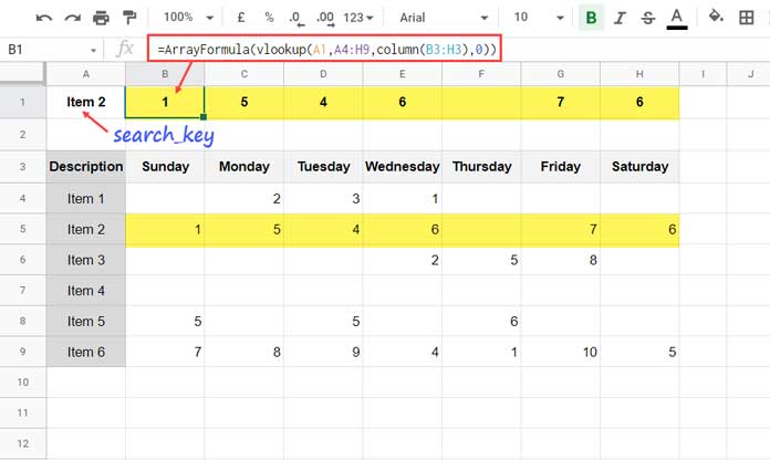
=ArrayFormula(vlookup(A1,A4:H9,column(B3:H3),0))In this formula, the search_key is located in cell A1, the range to lookup is A4:H9 (the first column contains the search_key), and the index is set to columns 2 to 8. As a result, the formula returns a 7-column result.
Now that we have a basic understanding of Vlookup result columns, let’s explore how we can filter them to meet various requirements.
Example: Filtering Vlookup Result Columns in Google Sheets
In the following examples, we will walk you through different scenarios where you may need to filter Vlookup result columns to achieve specific outcomes.
Filter Out Blanks from Vlookup Result Columns
Suppose you want to filter out any blank cells in the Vlookup result. By using the Filter function, you can easily achieve this. Let’s say we replace the search_key in cell A1 with “Item 3”. The master formula would return the following result:
2 5 8To filter out the blank cells, simply apply the Filter function as follows:
=filter(
     vlookup(A1,A4:H9,column(B3:H3),0),
     len(vlookup(A1,A4:H9,column(B3:H3),0))
)
This formula filters out the blank cells using the len function. It’s a handy trick when you only want to retrieve results from the first ‘N’ non-blank columns in the Vlookup. To achieve this, you can include Array_Constrain as well:
=array_constrain(
     filter(
        vlookup(A1,A4:H9,column(B3:H3),0),
        len(vlookup(A1,A4:H9,column(B3:H3),0))
     ),1,N
)
Replace ‘N’ with the desired number, such as 1 for the first value, 2 for the first two values, and so on. This method is particularly useful if you previously used a nested Vlookup formula to retrieve the first non-blank value after a vertical lookup, as shown here.
Applying Comparison Operators
Another advantage of combining Filter with Vlookup is the ability to apply comparison operators. Let’s say you want to lookup “Item 6” in column A and return only the sales values less than 5. To achieve this, you can use the following formula:
=filter(
     vlookup(A1,A4:H9,column(B3:H3),0),
     vlookup(A1,A4:H9,column(B3:H3),0)<5
)
This formula filters the Vlookup result columns based on the specified condition. It’s a powerful technique that allows you to fine-tune your results.
Filter Vlookup Result Columns to Remove Unwanted Values
To further refine your Vlookup result, you can use additional comparison operators or regular expressions. Here are three examples to illustrate this:
Example #1: Filter for Values Not Equal to 5
=filter(
     vlookup(A1,A4:H9,column(B3:H3),0),
     vlookup(A1,A4:H9,column(B3:H3),0)<>5
)
Example #2: Filter for the Value 5
=filter(
     vlookup(A1,A4:H9,column(B3:H3),0),
     vlookup(A1,A4:H9,column(B3:H3),0)=5
)
Example #3: Advanced Filtering Using Regexmatch
=filter(
     vlookup(A1,A4:H9,column(B3:H3),0),
     regexmatch(vlookup(A1,A4:H9,column(B3:H3),0)&"", "^1$|^10$")
)
The third example demonstrates how to use Regexmatch to filter Vlookup result columns using multiple conditions. If the result columns contain text, you can replace the values 1 and 10 with the corresponding strings. For more information on using Regexmatch in filter criteria, check out our guide here.
You can add more conditions by separating them with a pipe delimiter, such as ^apple$|^orange$|^banana$. To return values that are not equal to 1 and 10 after a Vlookup, use the FALSE Boolean:
=filter(
     vlookup(A1,A4:H9,column(B3:H3),0),
     regexmatch(vlookup(A1,A4:H9,column(B3:H3),0)&"", "^1$|^10$")=FALSE
)
Filtering Vlookup Result Columns and Handling N/A Errors
In some cases, the above formulas may result in #N/A errors. This can happen when the Vlookup search_key is not present in the first column or when the Filter function doesn’t find a match. To handle these errors and display a custom value instead, you can wrap the outer formula with IFNA:
=ifna(formula,"message")That’s it! You are now equipped with the knowledge to filter Vlookup result columns in Google Sheets like a pro. Start exploring the possibilities and unleash the true potential of your data.
For more expert tips and tutorials, visit Crawlan.com. Happy filtering!


