Applying a date filter in a Gantt Chart is tricky in Google Sheets. You may often require it to see tasks in a defined window of time (time frame). So you will get larger bars due to the shorter period. Also, it will help you find the tasks starting or in progress from the selected start date or within the defined time frame. What about using Data > Create a filter to filter the tasks based on the start date? That won’t yield the required output. Because that may hide some tasks (rows). Can you explain it? Yep! My source data is in the following format – Task Name (A), Duration (B), Start (C), and End (D).
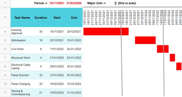
Assume one of my tasks, i.e., “Drawing Approval” starts on 15-11-2021 and ends on 20-12-2021. I want to see the tasks in the time frame, i.e., from 15-12-2021 to 14-01-2022. If I filter column E (Start) for dates >= 15-12-2021, the row containing the task name “Drawing Approval” will become hidden. But I want to see its bar from 15-12-2021. This post explains how to get a proper date filter in a Gantt Chart in Google Sheets.
Utilisation de Sparkline Bar pour limiter la vue du diagramme de Gantt à certaines dates
Since there is no predefined Gantt chart type in Google Sheets, we can create one using conditional formatting, Sparkline, or Stacked Bar chart. We can rely on Sparkline to get the date filter in a Gantt chart because the other two won’t suit our purpose. If we use conditional formatting, we may require to use days as the unit in the timescale to get a proper chart. This type is only suitable for a project with a shorter period. At present, we can’t use the date filter in a Stacked bar Gantt Chart also. Here, we may be required to edit the chart each time to enter the Min value on the X-axis.
Comment obtenir un filtre de date dans un diagramme de Gantt dans Google Sheets
We will start with the sample data. Copy-paste the below sample data in A3:D11. There are three main steps. They are the formulas for the duration in B4, Timescale in E3, and Gantt Bar in E4:E11.
Formules – Durée, Plage de temps et Sparkline
1. Durée
Empty the duration column range B4:B and insert the following array formula in cell B4.
=ArrayFormula(if(D4:D="",,days(D4:D,C4:C)))
2. Plage de temps (Filtre de date dans le diagramme de Gantt)
It plays a vital role in applying the date filter in the Gantt Chart in Google Sheets. First, we require to define the window of time to limit the Gantt Chart view.
In cell C1, enter the start date to filter. For the time being, input 15-11-2021 in it.
In cell D1, we will apply a data validation rule. Go to Data > Data validation > Criteria > Custom formula is. Insert the following formula and Save.
=and(D1>C1,isdate(D1))
The above validation makes sure that the D1 date is greater than the C1 date.
Enter 31-03-2022 in cell D1.
The following SEQUENCE formula in cell E3 will return the required time frame.
=sequence(1,60,C1,ROUNDUP(days(D1,C1)/60))
Select the entire columns E3:BL3. Right-click and select “Resize columns E – BL” and enter 16 (pixel) as the width of the columns. You can set it as per your requirement.
The above is one of the main formulas in getting the date filter in our Gantt Chart as it dynamically adjusts the timescale units based on the time frame in C1:D1.
3. Sparkline Bar Chart with Date Filter
Select E4:BL4 and go to Format > Merge > Merge horizontally. Now here is the SPARKLINE function-based formula to draw the Gantt Chart.
=sparkline( {min(max(C11,$C$1),$BL$3)-$C$1,max(min(D11,$BL$3),$C$1)-min(max(C11,$C$1),$BL$3)}, {"charttype","bar";"color1","white";"color2","red";"max",$BL$3-$C$1} )
It will adjust along with the timescale based on the given time frame. Copy-paste it down.
Follow the above steps to get a date filter in a Gantt Chart in Google Sheets.
Formule (Sparkline) Explication
Generic Formula: sparkline( {task_start-project_start, task_end-task_start}, {« charttype », »bar »; »color1″, »white »; »color2″, »red »; »max »,duration} )
task_start (not C4) = min(max(C4,$C$1),$BL$3)
project_start = $C$1
task_end (not D4) = max(min(D4,$BL$3),$C$1)
task_start = min(max(C4,$C$1),$BL$3)
The total project ‘duration’ is not $D$1-$C$1, but $BL$3-$C$1.
If you fail to create a date filter in Gantt Chart as above, feel free to copy my template below.
Thanks for the stay. Enjoy!
Visit bolamarketing.com for more exciting articles like this.

