Imagine being able to create grid charts to better understand data and get an overview at a glance. In this article, I’m going to show you how to easily create a grid chart in Google Sheets.
Grid charts are an excellent way to visualize the distribution of a whole into its constituent parts. They allow you to quickly see the different proportions and understand the overall situation.
Creating a Grid Chart in Google Sheets
Follow these simple steps to create your own grid chart in Google Sheets:
1. In cell A1, enter a percentage value, for example, 73%.
2. Below that, in cell A3, enter the following SEQUENCE formula:
=SEQUENCE(10,10)
This generates a grid of ascending numbers from 1 to 100.
3. Adjust the column widths (and row heights) so that the cells are square.
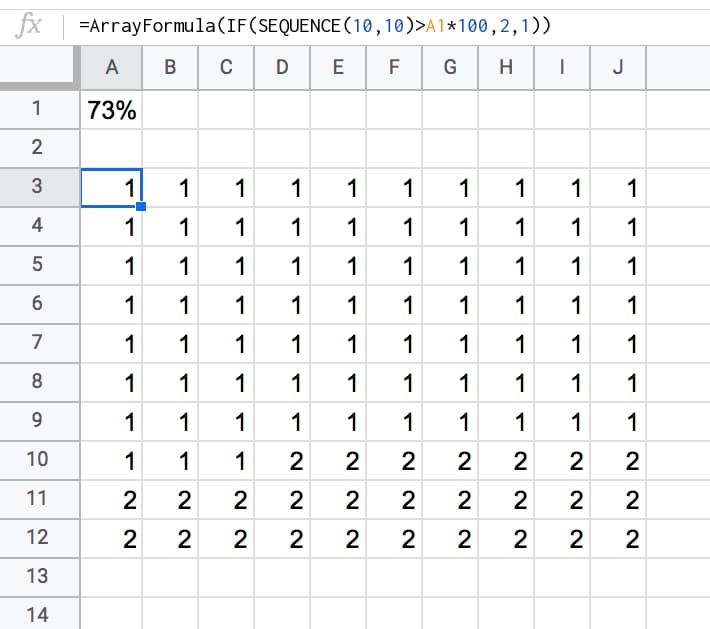
4. Wrap the SEQUENCE function with an IF statement and ArrayFormula to check if the value in a given cell is greater than the threshold percentage. For example:
=ArrayFormula(IF(A3:J12>$A$1,1,2))
Your result will look like this:
5. Highlight the 10 by 10 grid and add two conditional formatting rules:
- Green background if the value “equals 1”
- Gray background if the value “equals 2”
6. With the 10 by 10 grid highlighted, add thick white borders to separate the grids. Also, disable gridlines for a cleaner appearance.
7. Keep the highlighted grid, change the number format to a custom number format with the emoji symbol: 👤
Format > Number > More Formats > Custom number format, then paste the emoji: 👤
This will change all values to 👤, whether it’s a 1 or a 2.
8. Finally, center the values horizontally and vertically.
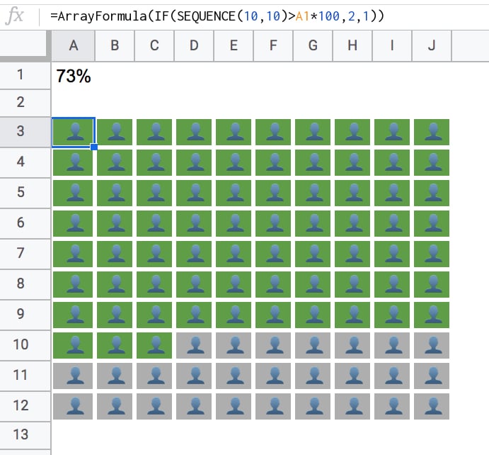
And there you have it! When you modify the percentage value, the chart will automatically adjust for you.
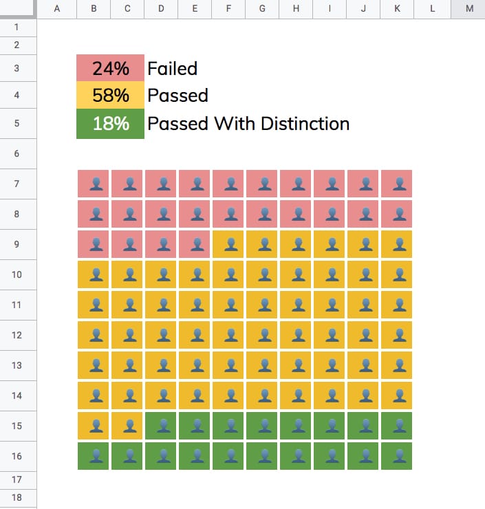
3-Color Grid Chart
To create a 3-color grid chart like this:
Add an additional percentage value and modify the formula to compare the two percentages using two IF statements, for example:
=ArrayFormula(IF(A3:J12>$A$1+percentage,1,IF(A3:J12>$A$2,2,3)))
You will also need to add an additional conditional formatting rule for cells with the value 3.
Google Sheets Grid Chart Template
Click here to open the Google Sheets Grid Chart template.
This will open a read-only version of the template. Feel free to make a copy: File > Make a copy
(If you’re unable to open this file, it may be because it’s from an external organization and my G Suite domain is not whitelisted by your organization. You can ask your G Suite administrator about this. In the meantime, feel free to open it in a private browsing window to view it.)
Now that you know how to create a grid chart in Google Sheets, explore the possibilities and use them to visualize your data in a clear and concise manner. Enjoy this trick and share it with your friends!
For more tips and advice on Google Sheets, visit Crawlan.com.
Article based on the original by Ben Collins: How To Create A Grid Chart In Google Sheets


