Do you want to efficiently organize and manage your data in Google Sheets? Look no further! In this article, we’ll dive into the world of tables in Google Sheets, also known as “Array Literals.” These collections of data, composed of rows and columns, can be used in formulas just like regular ranges.
Creating Tables in Google Sheets
Let’s start with a simple example of a row table:
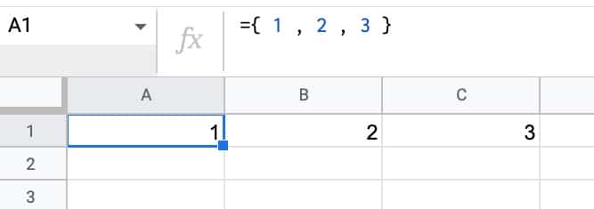
To create this table in cell A1, simply use the following formula:
{1, 2, 3, 4, 5}The opening and closing braces denote the table, while the commas separate the data into columns. (Note: European users might need to use semicolons as column separators due to syntax differences in Google Sheets.)
Now, let’s explore a column table:
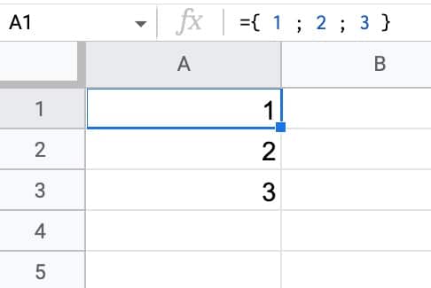
The formula for this table is:
{1; 2; 3; 4; 5}In this case, semicolons create new lines in the table.
For a two-dimensional table example:
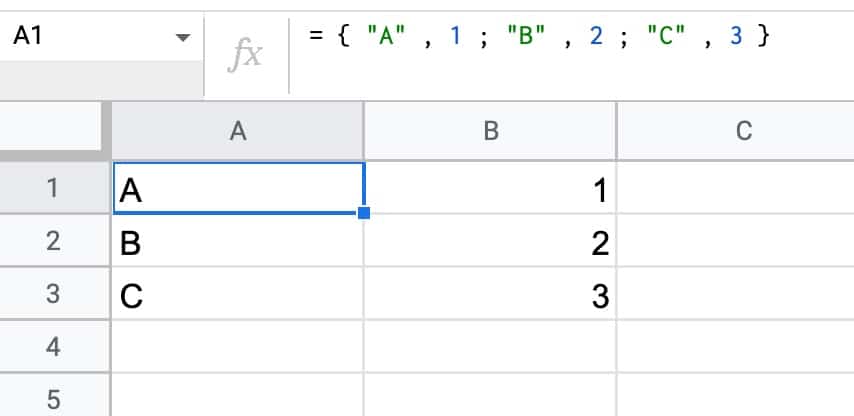
Entering the following formula in cell A1 creates a 3×2 table, filling the range A1:B3:
{{1, 2}, {3, 4}, {5, 6}}You can observe the combination of braces to create the table, commas to create columns, and semicolons to create new lines.
Notes on Array Literals
Array Literals are not limited to just numbers or strings. You can also nest formulas or even table formulas within the braces, unlocking their full potential. Additionally, you can use the outputs of arrays as inputs for other formulas.
For more information on using Array Literals, consult the Google Sheets documentation. Keep in mind that there are other ways to generate arrays, such as using the SEQUENCE function to generate data ranges in rows, columns, or two-dimensional format.
Practical Examples of Tables in Google Sheets
Now that you know how to create tables, let’s explore some practical applications using formulas.
Returning Multiple VLOOKUP Columns
Traditional VLOOKUP formulas limit you to returning a single column. However, by nesting an Array Literal as the column index, you can retrieve multiple columns at once.
Take a look at this example:
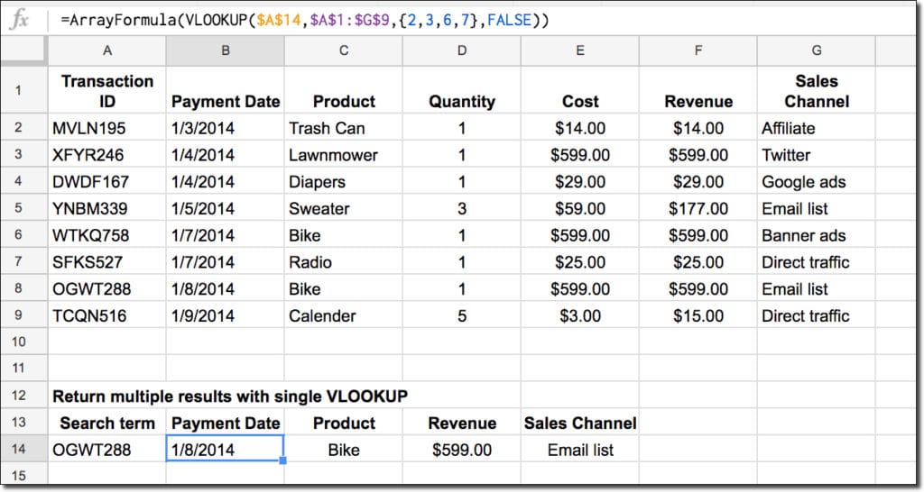
Notice the nested Array Literal in the VLOOKUP formula, indicated in red:
=VLOOKUP(A1, {A1:D10, G1:H10}, {2, 3, 6, 7}, 0)This VLOOKUP will simultaneously return results from columns 2, 3, 6, and 7.
Combining Formulas with Tables in Google Sheets
One notable difference between the powerful QUERY function and a pivot table is that QUERY does not automatically add a grand total row. However, you can use tables in Google Sheets to easily add a dynamic grand total row.
Essentially, you combine the results of the QUERY function with the SUM function:
=QUERY(A1:B6, "SELECT A, SUM(B) WHERE A IS NOT NULL GROUP BY A WITH ROLLUP")This formula will display a table like this in your Google Sheet:
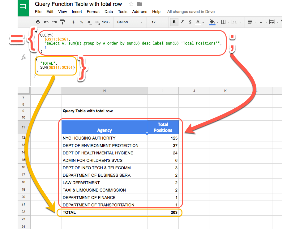
To learn more about adding a grand total row to a QUERY table in Google Sheets, refer to the documentation.
Setting Default Cell Values in Your Google Sheet
Did you know that you can use tables in Google Sheets to create default values for cells?
Array Literals create a formula that propagates to adjacent cells, allowing you to set default values. Here’s an example:
In an empty sheet, enter the value “Entry” in cell A1. Then, in cell B1, type the following formula:
=ARRAYFORMULA(IF(ISBLANK(A1), 100, A1))Your spreadsheet will look like this:
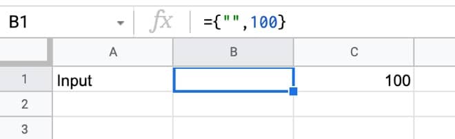
Try entering “200” in cell C1, overwriting the default value of “100”. Cell C1 will display “200,” but cell B1 will show an error (#REF!).
Now, delete the value you just entered in cell C1. The error message will vanish, and the default value of 100 will reappear in cell B1.
For a cleaner look, hide column B, so the #REF! error is never visible. You will then have a default value of 100 set for cell C1.
To learn more about default values in Google Sheets and discover an advanced method for creating default values without the need for a hidden column, visit the Crawlan.com website.
With these table techniques in Google Sheets, you’ll be able to organize your data efficiently and harness the full potential of formulas.
So, why wait? Start creating dynamic tables in Google Sheets today with Crawlan.com!


