How to Create a Dynamic Chart Title from a Cell Value in Google Sheets

Discover how to create a dynamic chart title linked to a cell in Google Sheets in this tutorial.

Graphs are excellent tools for visualizing data. They are widely used because they are simple and easy to understand. With the exception of the title section, almost all other parts of a chart in Google Sheets are highly customizable and dynamic.

This post will show you how to create a dynamic chart title in Google Sheets using values from a specific cell.

Linking a Chart Title to a Cell to Make It Dynamic

Chart titles are very important. They help users get a quick summary of the chart’s content and make understanding easier. In Google Sheets, you can add chart titles using the title placeholder when creating the chart. However, this solution is static and does not automatically update if you change your data.

Having a dynamically changing chart title can give your chart an extra functionality. This is especially handy when you have a chart that is frequently updated with new data. As the underlying data gets updated, the information on the chart will likely change and, consequently, your chart title should reflect the new perspective.

Finding a native solution in Google Sheets that allows dynamically changing a chart title can be difficult, if not impossible. But fret not because we have created a custom solution using Google Apps Script.

Example Data

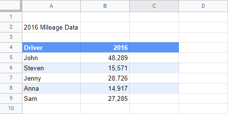
Before using the script, start by inserting a chart. Our example data contains information about specific drivers’ mileage for the year 2016.

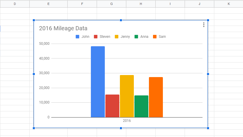
And here’s the chart that visualizes the data:

When the chart updates with the 2017 data, you can use an Apps Script solution to change the chart title based on the values of a cell following these steps.

Step 1. Open the Google Apps Script Editor

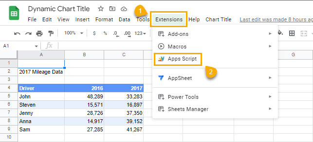
To open the Google Apps Script editor, follow these steps:

1. Click on the Extensions menu.
2. Select Apps Script from the dropdown options.

Step 2. Create a Custom Apps Script Function

When the Google Apps Script editor opens, copy and paste the code below.

function onEdit(e) {
  var sheet = SpreadsheetApp.getActiveSheet();
  var range = e.range;
  var activeColumn = range.getColumn();
  var activeRow = range.getRow();
  if (
    activeColumn == 1 &&
    activeRow == 1
  ) {
    var newTitle = sheet.getRange(activeRow, activeColumn).getValue();
    var charts = sheet.getCharts()[0];
    var chart = charts.modify()
      .setOption('title', newTitle)
      .build();
    sheet.updateChart(chart)
  }
}

After pasting the code in the editor, perform the following steps:

1. Click on the Save command.
2. Click on Run.

When you click the Run command, you will be prompted to grant certain permissions before the script can run.

This script creates a function called onEdit(e). To understand how it works, here’s an explanation of each line of code in the script:

• function onEdit(e) { }: This first line of code creates and names the function using the “function” keyword. The “function” keyword has the following syntax:

  function <function-name>() {
    // code to execute
  };

  Using this syntax, the “function” keyword defines this Apps Script. In the <function-name> parameter, we have “onEdit(e)”. While “onEdit(e)” names the function, “onEdit(e)” is a trigger.

  Triggers are keywords that allow functions to automatically run when certain events occur. The “onEdit(e)” trigger executes the function when you modify the content of a cell in the spreadsheet.

• var sheet = SpreadsheetApp.getActiveSheet(): This creates a variable called sheet. The variable acts as a container that stores the currently active spreadsheet.

• var range = e.range: The range variable stores the range of cells where the edit event occurred.

• var activeColumn = range.getColumn(): getColumn() is a method that returns the index of the first column in a range. In this case, it will return the column number of the modified cell.

• var activeRow = range.getRow(): The getRow() method, much like the getColumn() method, returns the index of the first row in a range. Similarly, it will return the row number of the modified cell in this script.

• if (activeColumn == 1 && activeRow == 1) { }: This code forms the condition parameter to be tested. Essentially, it checks if the value of the activeColumn variable is equal to 1 and if the value of the activeRow variable is equal to 1. The implication of this condition is that only modifications made to cell A1 will directly affect the chart title in the spreadsheet.

• var newTitle = sheet.getRange(activeRow, activeColumn).getValue(): The getRange() method returns the range of a given cell. Its syntax getRange(row, column) takes a row and column index and returns a specific range.

  In this code, the activeRow and activeColumn variables are used to provide the row and column arguments in the getRange() method. Since this code block only runs when the activeRow and activeColumn variables are both equal to one, the getRange() method will return cell A1.

  The getValue() method returns the content of a given cell. In this code, it will return the content of cell A1. This value is stored in the variable named newTitle.

• var charts = sheet.getCharts()[0]: The getCharts() method returns an array of all charts in the active spreadsheet. sheet.getCharts()[0] returns the first chart in the active spreadsheet, which is stored in the variable called charts.

• var chart = charts.modify(): The modify() method allows making modifications to specific sections of the chart by creating a built-in chart builder that is used to modify a chart. With this line of code, you can choose which part of the chart to modify.

• .setOption('title', newTitle): While the previous code allows you to modify the chart, this method allows you to select which part of the chart you want to modify and what type of modification you want to make. The setOption() method has two parameters. The first parameter refers to the part of the chart you want to modify, while the second parameter refers to the code containing the type of modification you want to make. In this case, the chart title will be modified using the values from the newTitle variable.

• .build(): Once all the modifications have been made, this method creates a new chart and applies all the specified modifications in the preceding codes. All of this is stored in the variable chart.

• sheet.updateChart(chart): This code applies all the modifications created in the chart variable to the selected chart in the active spreadsheet.

When you execute this code in the Google Apps Script editor, you’ll get a runtime error message.

When this happens, there’s no need to worry as the script will work perfectly fine. This happens every time the onEdit(e) trigger is used in a script. The reason for this error is that the edit event doesn’t exist yet, causing the engine to read the range variable as undefined.

Once you’ve pasted and saved this script in the editor, go back to your spreadsheet and refresh it.

Step 3. Run the Script to Dynamically Change the Chart Title

Since the sample data has only contained information for the year 2016 until now, when the 2017 data is added to the chart, you can change the chart title by simply updating the content of cell A1.

This solution opens up many other possibilities. You can link the title cell to another cell or use data validation.

To learn more about advanced features in Google Sheets, visit Crawlan.com.