Google Sheets is not just a basic spreadsheet program; it is packed with advanced features that can help you make sense of your data. One of the most useful and powerful features is conditional formatting. This feature allows you to transform plain black text on a white background into a visually appealing and colorful set of data. Not only does this save time, but it also makes your data more readable and meaningful.
In this article, we will dive into the world of conditional formatting in Google Sheets and show you how to take advantage of this incredible tool. Whether you’re a beginner or an experienced user, you’ll find valuable tips and tricks to make your data shine.
What is Conditional Formatting in Google Sheets?
Conditional formatting in Google Sheets is a feature that automatically changes the appearance of a specific cell, row, column, or even the background color of the cell based on the rules you set. In other words, it allows you to visually highlight specific values in your data, making them easier to understand and analyze.
By using conditional formatting, your data becomes not only visually appealing but also more readable to humans. You can easily spot trends, outliers, and patterns in your data, making it easier to draw insights and make informed decisions.

When Can You Apply Conditional Formatting in Google Sheets?
Conditional formatting can be applied in virtually any scenario where you need to visualize information. It’s a versatile tool that can be used in various workflows to highlight data patterns, identify problem areas, showcase positive trends, or even flag erroneous or faulty data.
Here are a few examples of how different professionals can leverage conditional formatting in their work:
- Sales managers can quickly extract insights from a large amount of sales data by using conditional formatting.
- Accountants can easily highlight negative values in red in their profit/loss calculations.
- Project managers can understand resource utilization and identify bottlenecks using conditional formatting.
Conditional formatting is also an effective tool for tracking progress towards specific goals. Whether you’re monitoring sales targets, website traffic, or social media engagement, conditional formatting can provide visual indications of progress and keep you motivated.
In large organizations, daily and weekly reports are abundant. However, they can become overwhelming if they’re not conditionally formatted. By applying conditional formatting, you can make these reports more meaningful and immediate, saving precious time and effort.
As you can see, conditional formatting can be useful in a wide range of scenarios, bringing your Google Sheets tables to life.
How to Use Conditional Formatting in Google Sheets
Now that you understand the power of conditional formatting, let’s dive into the practical steps to apply it in your Google Sheets.
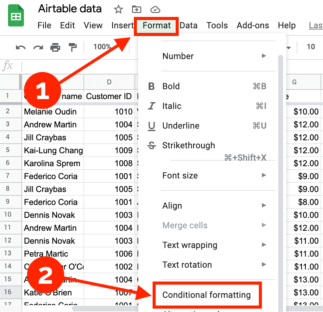
Step 1: Click on “Format” -> “Conditional formatting”
The first step is simple and straightforward. Just navigate to the “Format” menu in Google Sheets and click on “Conditional formatting.”
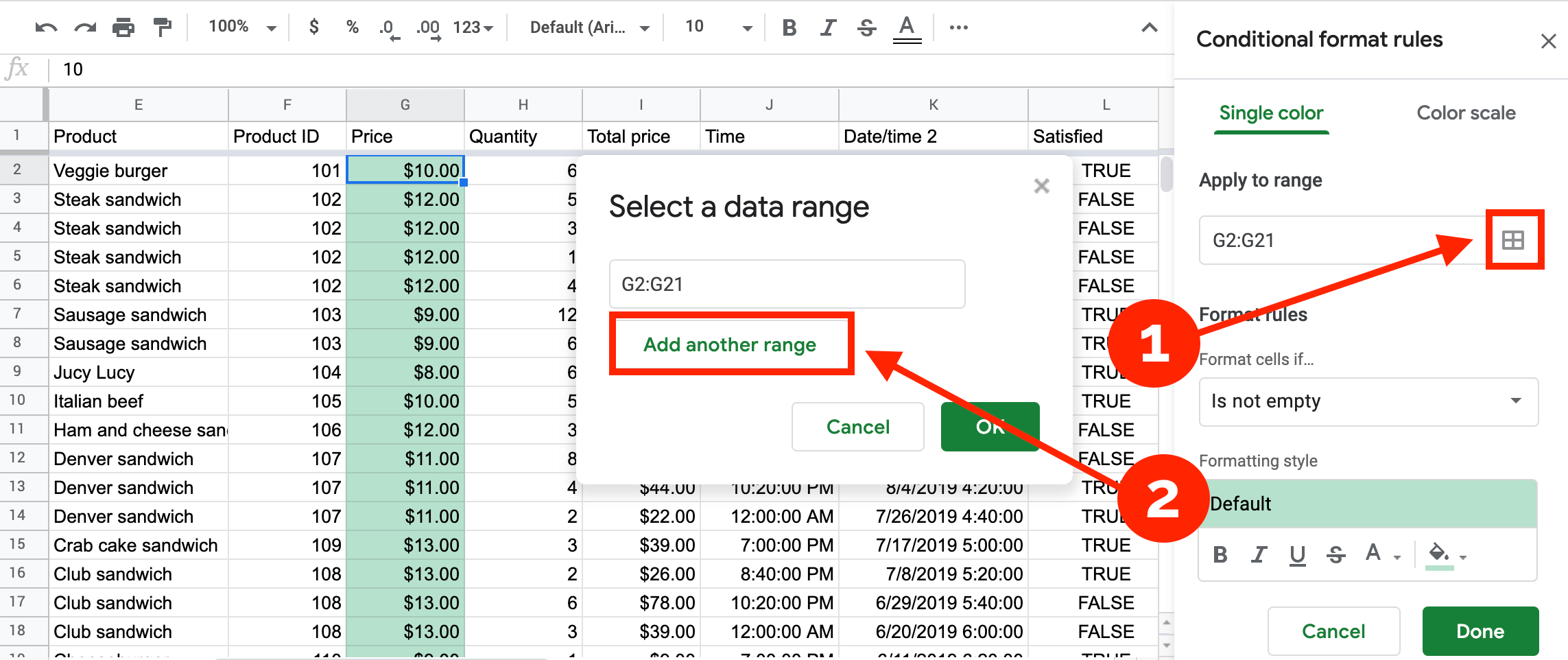
Step 2: Select a Range
In the second step, you need to select the range of cells, columns, or rows to which you want to apply the conditional formatting. You have two options here:
- Option 1: Select the range directly (cells, columns, or rows) and then click on “Format” -> “Conditional formatting.” This will bring up a conditional formatting toolbar on the right side of your screen. This option is ideal for small data ranges.
- Option 2: Click on “Format” -> “Conditional formatting” and then enter your range in the “Apply to range” tab. This method is particularly useful when working with large amounts of data to avoid any potential mistakes in range selection.

Make sure to specify the range correctly. For example, if you want to highlight a single cell, enter the cell label (e.g., G2). If you want to target a range of cells, separate the first and last cell with a colon (e.g., G2:G21 in the above example).
You can also work with multiple ranges by clicking on the icon to the right of the range field and selecting “Add another range.” This feature allows you to highlight as many ranges as you want.
Step 3: Define Conditional Formatting Rules in Google Sheets
Now, let’s dive into the exciting part: defining the rules for conditional formatting. Every conditional formatting follows the same pattern, which consists of three key elements:
- Range: This refers to the cell or cells to which the rule should be applied.
- Trigger: The trigger sets the condition for the rule to be applied. For example, the trigger can be “Less Than” or “Equal To.”
- Style: This determines how the cell’s appearance will change when the rule is applied.
-
Format Style: Start by selecting the style for your conditional formatting. You can choose from the predefined styles or create a custom style that suits your needs. The style determines how the cell will look when the condition is met.
-
Format Cells If…: After selecting the style, you need to define the condition or trigger for the rule. Click on the “Format cells if…” drop-down list to see a wide range of triggers you can choose from. For example, you can select “Greater Than” or “Less Than” to highlight cells based on numerical values.
-
Apply the Rules: Once you’ve selected the style and trigger, click “Done” to apply your rules. You can always come back and modify the rules or add new ones to fine-tune the conditional formatting.
Now that you know the basic steps, let’s take a closer look at each one using a real-life example.
Step 1: Click on “Format” -> “Conditional formatting”
Clicking on the “Format” menu and selecting “Conditional formatting” will open the conditional formatting toolbar.
Step 2: Select a Range
Next, you need to select the range of cells to which the conditional formatting will be applied. You can either directly select the range or enter it manually in the “Apply to range” tab. Make sure to select the correct range, as this determines the scope of your conditional formatting.
Step 3: Define Conditional Formatting Rules in Google Sheets
The third step is where the magic happens. You can now define the rules for your conditional formatting. This involves selecting the style and trigger for the formatting.
To select a style, click on the “Format Style” drop-down menu and choose the style that suits your preferences. You can also create a custom style by selecting the font properties and colors manually.
For the trigger, click on the “Format cells if…” drop-down list and select the trigger that fits your needs. This can be anything from basic numerical comparisons to complex custom formulas.
Once you’ve defined the style and trigger, click “Done” to apply the conditional formatting rules. You can always go back and modify the rules or add new ones as needed.
Now that you know the basic steps, you’re ready to unleash the full potential of conditional formatting in Google Sheets. With a little creativity and experimentation, you can use conditional formatting to create visually stunning and insightful data presentations.
Advanced Tips and Tricks for Conditional Formatting
Conditional formatting in Google Sheets offers a wide range of possibilities. Here are some advanced tips and tricks to help you make the most out of this powerful feature:
- Text-Based Conditional Formatting: You can use text-based rules to find or highlight specific words or phrases in your data. This is great for analyzing text-heavy datasets or finding specific keywords.
- Conditional Formatting Based on Another Cell’s Value: Sometimes, you may want to apply conditional formatting based on the value of another cell. This can be done using custom formulas that reference other cells in your sheet. It allows for dynamic and flexible conditional formatting.
- Highlighting Entire Rows: If you want to highlight entire rows based on certain conditions, you can easily achieve this by adjusting the range for your conditional formatting. By selecting the entire row instead of a specific range of cells, you can highlight entire rows based on specific criteria.
- Custom Conditional Formatting: Google Sheets allows you to create custom formulas for conditional formatting. This gives you the flexibility to tailor the rules to your specific needs. You can use built-in functions like AND and OR to create complex conditions.
- Conditional Formatting for Dates and Time: You can apply conditional formatting to dates and time data in Google Sheets. This allows you to highlight past due dates, upcoming events, or any other time-related conditions.
- Conditional Formatting with Multiple Rules: Google Sheets allows you to set multiple conditional formatting rules for a single range. This can be useful when you have different conditions you want to highlight simultaneously.
- Highlighting Lowest or Highest Values: Conditional formatting can be used to highlight the lowest or highest values in your data. This can help you quickly identify outliers or focus on specific data points.
- Conditional Formatting with Checkbox: If you want to apply conditional formatting based on the status of a checkbox, you can achieve this by using custom formulas and the checkbox feature in Google Sheets.
- Conditional Formatting Across Different Sheets: Unfortunately, conditional formatting rules only apply to the tab in which they are entered. However, you can use the INDIRECT function to reference a different tab in your sheet and apply conditional formatting across multiple tabs.
- Troubleshooting Conditional Formatting: If your conditional formatting doesn’t work as expected, there could be several reasons. Pay attention to the order of your conditional formatting rules, ensure your formulas are correct, and be aware of any limitations or inconsistencies in conditional formatting behavior.
These are just a few examples of what you can achieve with conditional formatting in Google Sheets. The possibilities are endless, and with a little practice, you’ll become a conditional formatting master.
Conclusion
Conditional formatting is a game-changer when it comes to making your data visually appealing, meaningful, and easier to understand. By leveraging the power of conditional formatting in Google Sheets, you can easily highlight and analyze trends, patterns, and outliers in your data.
In this guide, we walked you through the basics of conditional formatting and provided advanced tips and tricks to help you make the most out of this feature. Remember to experiment, be creative, and have fun with conditional formatting. With practice, you’ll be able to transform your data into stunning visual presentations that tell compelling stories.
To learn more about Google Sheets and its powerful features, visit Crawlan.com.

