How to Remove Duplicates in Google Sheets and Highlight Duplicates in Google Sheets

Introduction:

Hey there, besties! Do you ever find yourself dealing with duplicate data in Google Sheets? It can be a major headache, right? Well, worry no more! In this article, I’ll show you not just one, but five awesome methods to remove duplicates and highlight them in Google Sheets. Trust me, these techniques will save you a ton of time and help you make more accurate decisions based on your data. So, let’s dive right in!

The Trouble with Duplicates

Duplicates are repeated occurrences of the same record in your data. And boy, can they cause a lot of trouble! It’s crucial to identify and eliminate duplicates in Google Sheets before diving into any data analysis. Let me give you an example. Imagine you have two identical customer transactions worth $5,000 each in your database. If you summarize your data without removing the duplicates, you might think you made $10,000 with that customer. But in reality, it’s only $5,000. See the problem? You could end up making decisions based on false data. That’s why spotting and removing duplicates is so important.

Method 1: Removing Duplicates with the Remove Duplicates Tool

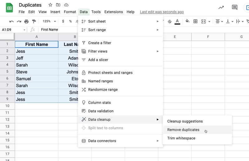
Let’s start with an easy method: the Remove Duplicates tool. You can find it in the menu: Data > Data cleanup > Remove Duplicates. When you click on “Remove Duplicates,” you’ll be prompted to choose the columns you want to check for duplicates. You can either remove duplicates when the entire rows are identical or select a specific column, like an invoice number, regardless of the data in other columns. The tool will then remove the duplicates and provide you with a summary report on how many duplicates were eliminated. It’s that simple! Check out the image below for a visual guide.

Method 2: Removing Duplicates with Formulas

If you’re dealing with smaller datasets or need to remove duplicates within a formula, the UNIQUE function is perfect for you. This function considers all columns in the data range to determine duplicates. In simple terms, it compares each row of data and removes any rows that are duplicates (identical to all other rows). The implementation is a breeze—all you need is a single formula with one argument: the range where you want to remove duplicates. Take a look at the example below:

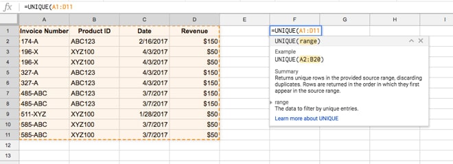
You can see that the table on the right has fewer rows because the duplicate rows have been removed. Super convenient, right?

Highlighting Duplicates with COUNTIF

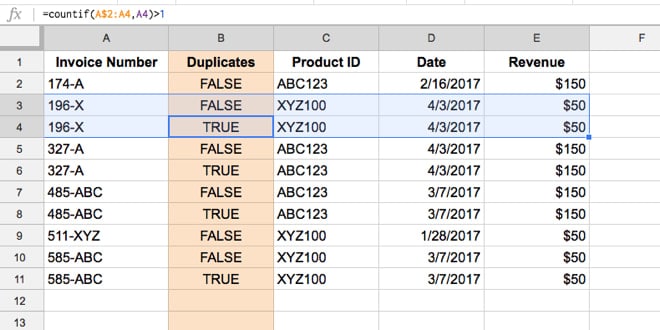
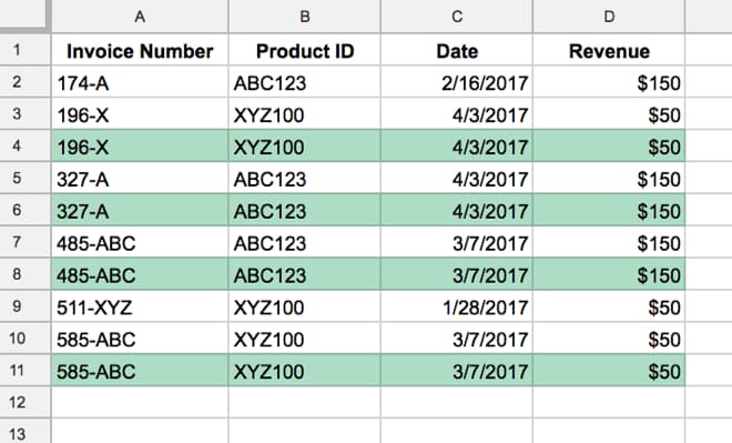
But wait, there’s more! If you want to highlight duplicates in Google Sheets, you can use the COUNTIF function. Here’s how it works: first, create a new column next to the column you want to check for duplicates (e.g., the invoice number). Then, use this formula in cell B2 to highlight duplicates in column A: =COUNTIF(A$2:A2,A2)>1. The $ sign is important here as it locks the top of the column range even when you copy the formula to column B. This formula checks for duplicates in the current row up until the top of the column. When a value appears for the first time, the count is 1, so the formula returns FALSE. But when the value appears a second time, the count is 2, so the formula returns TRUE. Finally, select the rows with TRUE values (the duplicates) and delete them. Check out the image below for a step-by-step visual guide.

Method 3: Finding Duplicates with Pivot Tables

Are you new to pivot tables? No worries! Pivot tables are fantastic for finding duplicates in Google Sheets and super easy to use. They’re incredibly flexible and quick, making them a great starting point if you’re unsure about the presence of duplicates in your data. Here’s how you can do it:

1. Select your data range and create a pivot table (in the Data menu).
2. A new tab will open with the pivot table editor.
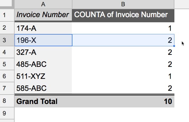
3. Under ROWS, choose the column you want to check for duplicates (e.g., the invoice number).
4. Under VALUES, choose another column (I often use the same one) and set it to be summarized by COUNT or COUNTA (if your column contains text).

The pivot table will then display the duplicates with a count greater than 1. From there, you can find these duplicate values in your original dataset and decide what action to take. Trust me, this method is the bee’s knees for finding duplicates in Google Sheets. Check out the image below for a visual reference.

Method 4: Highlighting Duplicates with Conditional Formatting

Ready for more awesome sauce? You can highlight duplicates in Google Sheets using conditional formatting. Here’s how:

1. Select your data range and open the conditional formatting sidebar (in the Format menu).
2. Under “Format cells if…”, choose “Custom formula” (the last option) and enter the following formula: =COUNTIF(A:A, A1)>1. This formula checks for duplicates in a single column, in this case, column A.
3. The result will be highlighting applied to the duplicate values. Sweet!

If you want to apply the highlighting to the entire row, modify the formula slightly by adding a $ sign before the last A: =COUNTIF($A:$A, A1)>1. Now your result will look like this, with the whole row highlighted:

For a more detailed guide on highlighting an entire row using conditional formatting, check out this article.

Method 5: Removing Duplicates with Apps Script

Feeling fancy? If you’re familiar with Apps Script, you can create a small program to remove duplicate rows from your data in Google Sheets. The beauty of writing a program with Apps Script is that you can run it over and over again, like a charm. Here’s an example of an Apps Script program that removes duplicates from a dataset in Sheet 1:

Code for removing duplicates with Apps Script

Impressive, isn’t it? This program works by:

1. Getting the values from the data range in Sheet 1 using Apps Script.
2. Converting the table rows into strings for comparison.
3. Filtering out the duplicate rows.
4. Checking if the deduplication sheet already exists.
5. If it exists, clearing out any previous deduplicated data and pasting the new deduplicated data.
6. If it doesn’t exist, creating a new sheet and pasting the new deduplicated data.
7. Adding a custom menu to run the program from the Google Sheet itself.

How cool is that? Apps Script allows you to quickly create custom solutions specific to your situation. Once you’ve mastered Apps Script, you can whip up custom scripts like this one in just 15 to 30 minutes. Talk about a time-saver!

Now that you know how to remove duplicates in Google Sheets using five different techniques, go ahead and banish those pesky duplicates from your datasets! Trust me, your future self will thank you.

And remember, if you ever need more Google Sheets tips and tricks, come visit us at Crawlan.com. We’ve got your back every step of the way!

Happy deduplicating, besties!