In this article, we will explore several ways to hide blank values in Google Sheets. We will also discuss a method that allows you to permanently delete blank values from your dataset. Keep reading to discover these methods in Google Sheets and get ready to apply them to your spreadsheet.
The Importance of Hiding Blank Values in Google Sheets
Google Sheets users often need to hide blank values in their dataset. The benefits of hiding blank values in Google Sheets highlight their significance and relevance.
Imagine you have a large and complex dataset. It would be difficult for you to quickly determine the cells that contain blank values. To make them more visible in your dataset, you can use formatting that replaces blank values with empty cells. This way, you can easily spot the empty cells that correspond to blank values in your dataset. Moreover, this won’t affect the formulas in your spreadsheet if you simply hide the blank values instead of deleting them permanently. So, it’s better to hide them for better visual interpretation.
Sometimes, blank values in your dataset simply indicate that the data is not available. In this case, it would be more appropriate to hide the blank values and display empty cells. Because, if you’re like me, you want a clean and organized spreadsheet and you want to hide something that may look incorrect. So, if you have data rows but some rows do not have data yet and you want them ready when that data is present, instead of displaying zero for each field without data, you can replace blank values with empty cells.
How to Hide Blank Values in Google Sheets
There are several logical methods to hide blank values in Google Sheets, including conditional formatting and custom formatting. However, these two methods only hide blank values without deleting them. We will also explore the method of removing blank values in Google Sheets.
This tutorial will guide you through the step-by-step procedures of each method to hide blank values in Google Sheets. Let’s get started!
Hide Blank Values in Google Sheets – Using Conditional Formatting
Conditional formatting is the method that allows you to format cells according to your needs. As we want to hide blank values, we can apply a condition stating that all cells containing blank values should be filled with the white color. This way, we can hide all the blank values in our data. Let’s see how it works.
Step 1
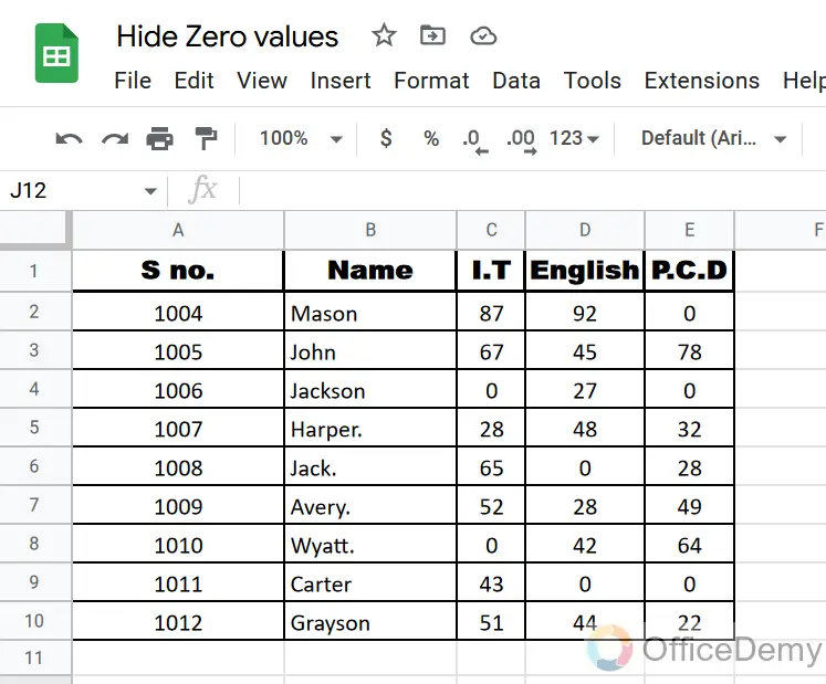
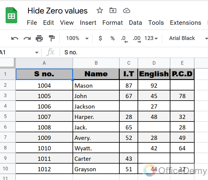
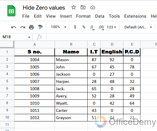
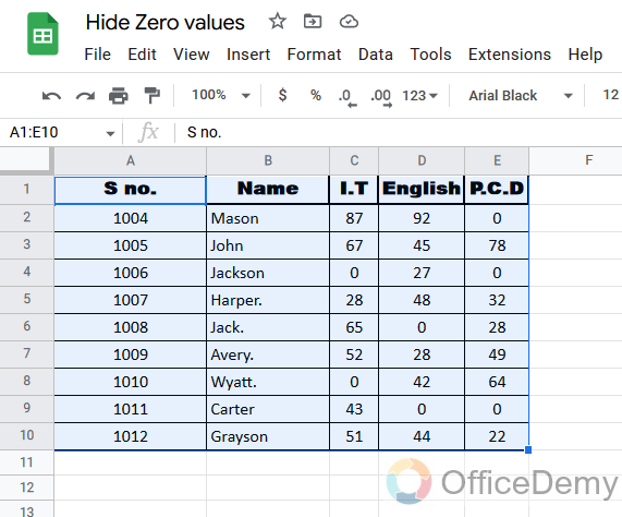
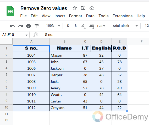
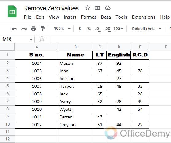
Start by having a sample data that contains multiple blank values.
Step 2
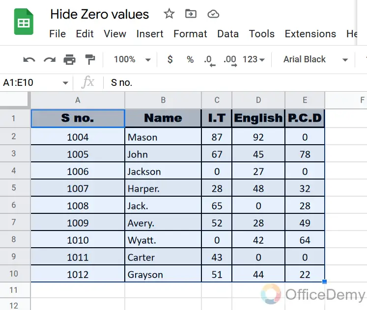
Select the range where you want to apply the formatting to hide blank values.
Step 3
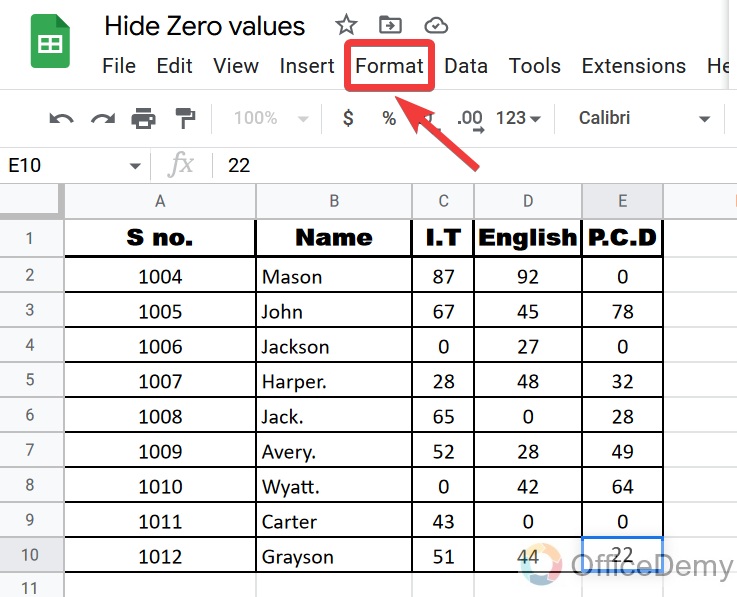
Now, look at the menu bar and open the “Format” option.
Step 4
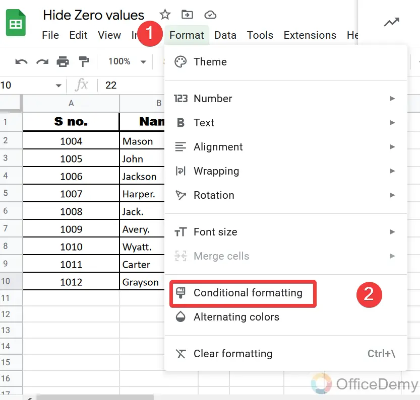
When you click on the “Format” tab, a drop-down menu opens where you will find the “Conditional formatting” option. Click to open it.
Step 5
Here, you need to change “Format cells if…” to “Equal to”. You may need to scroll a bit to see this option in the list.
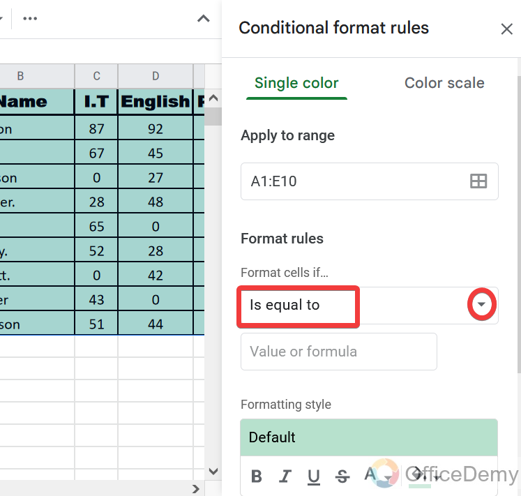
Step 6
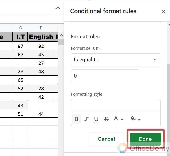
After selecting “Format cells if…”, an additional value box will appear where you need to put “0” as we are looking for blank values.
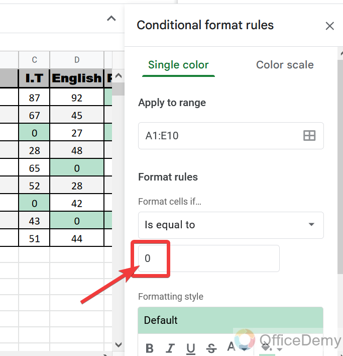
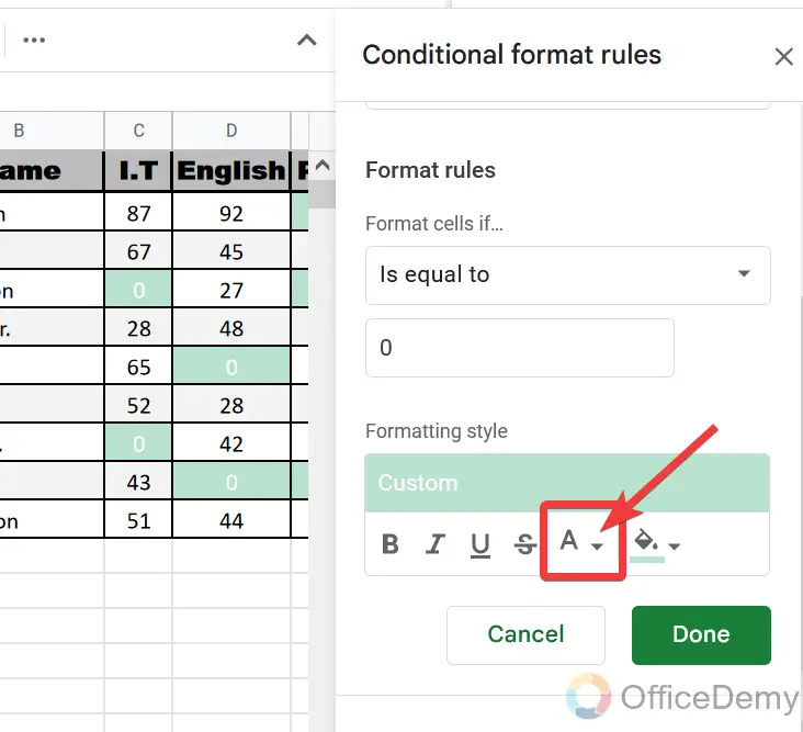
Step 7
When you give the condition, all the blank values will be automatically selected. We will now apply formatting to hide them. First, change the text color to “white” from here.
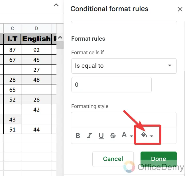
Step 8
Now, we will also change the cell background color to “white”.
Step 9
You’ve completed the formatting, just click on the “Done” button.
Step 10
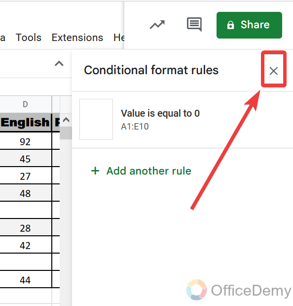
Now, you can close the conditional formatting pane.
Step 11
As you can see, all the blank values have been hidden.
Note: By applying the above method, blank values are only hidden, they are not deleted and still exist in their cells.
Hide Blank Values in Google Sheets – Using Custom Formatting
The previous method works well, but it doesn’t actually hide blank values, it just gives the illusion that they are hidden. To completely hide blank values, we will use custom formatting. In Google Sheets, custom formatting is based on a default text pattern. The pattern consists of sections for positive numbers, negative numbers, blank values, and text. According to this pattern, we will use the following format to hide blank values:
0;-0;;@
- Positive Number: They will remain the same as positive numbers using 0.
- Negative Numbers: They will remain the same as negative numbers using -0.
- Blank Values: We will leave the space empty instead of blank values to hide them.
- Text: We will display the text as it is, specified by the @ symbol.
Let’s see how to apply it in practice.
Step 1
As usual, start by having a sample data.
Step 2
Select all the data where you want to hide blank values.
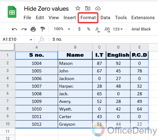
Step 3
After selecting the data, find the “Format” tab in the menu bar and open it.
Step 4
When you open the format tab, a drop-down menu appears where you will find “Number”.
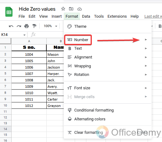
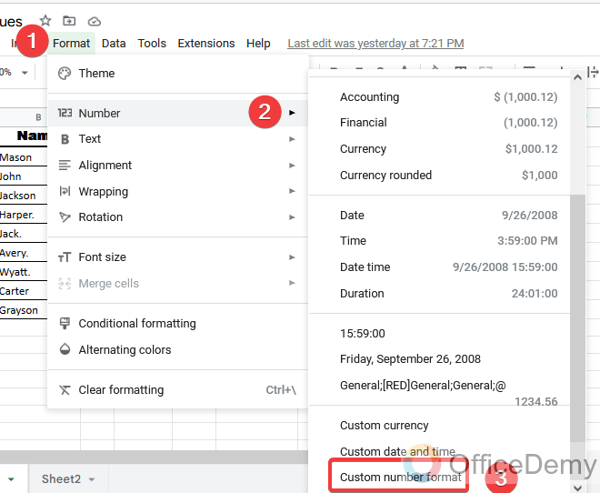
Step 5
Go to “Number”, a second menu will appear where you will find “Custom number format” by scrolling down.
Step 6
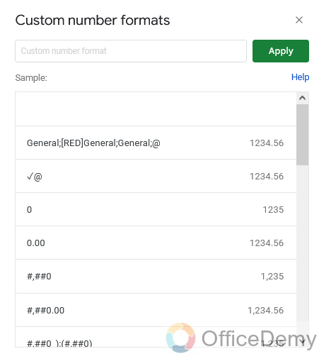
When you click on “Custom number format”, a new window appears in front of you like this:
Step 7
We will put the format (0;-0;;@) in the custom format dialog box that we created above to hide blank values.
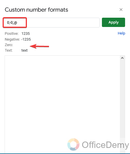
You can also check the format by looking at the format of all the values next to the format dialog box, as shown in the above image, there is a space for blank values, which means they will be hidden.
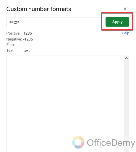
Step 8
Now, you’re just one click away from finishing your process. Click on the “Apply” button.
Step 9
As you can see below, all the blank values have been hidden.
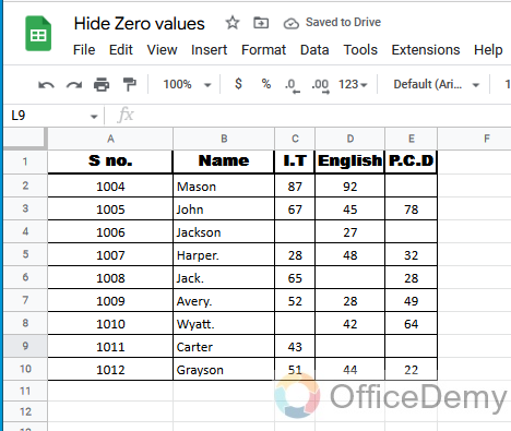
This method also hides blank values. It does not delete them.
How to Hide Blank Values in Google Sheets – Using the “Find and Replace” Function
We have discussed two methods so far, but both only hide blank values in Google Sheets. If you want to delete blank values, you can use the “Find and Replace” function of Google Sheets. This will first find all the blank values and then delete them. Let me show you how to remove blank values with the “Find and Replace” function using a few examples.
Step 1
Firstly, we are going to select the data where we want to delete blank values.
Step 2
Now, we will open the “Edit” tab in the menu bar, where you will find “Find and Replace” at the very bottom.
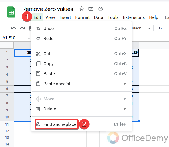
You can also use the shortcut “Ctrl + H” to open the find and replace dialog box.
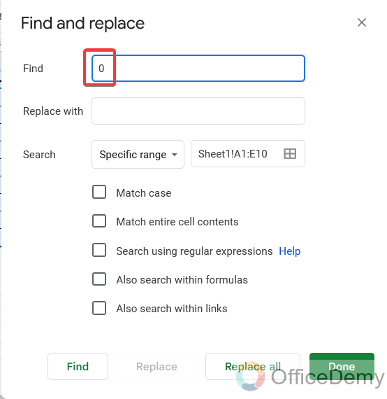
Step 3
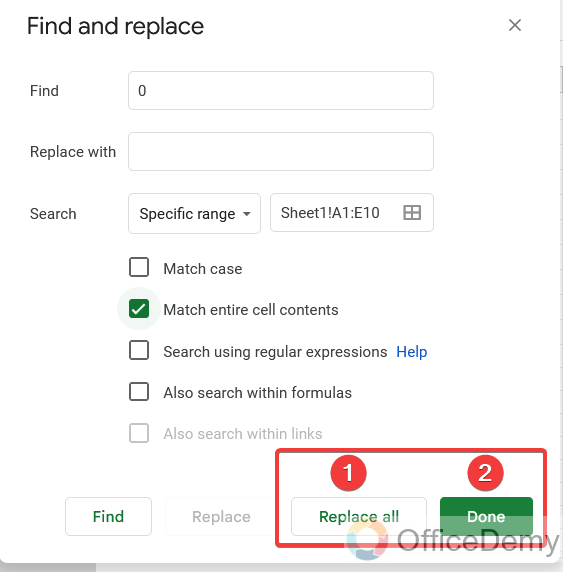
When you click on the “Find and Replace” option, a dialog box opens for finding and replacing values. So, as we are looking for blank values, we will put “zero” in the search box.
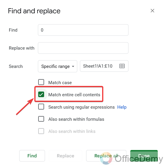
Step 4
Next, to delete them, leave the replacement box empty and check “Match entire cell contents”.
Step 5
Now, you just need to click on “Replace all” and then the “Done” button.
Step 6
You are done now. As you can see, all the blank values have been deleted.
Important Notes
Frequently Asked Questions
Can I use the same methods to hide blank values in Google Sheets when finding absolute value?
To hide blank values in Google Sheets when calculating absolute value, you can use the same methods. By applying conditional formatting rules, you can create a custom formula that targets cells containing blank values and hides them. This ensures that your absolute value calculations in Google Sheets appear cleaner and more organized.
Conclusion
Your priority is to make your documents, presentations, tables, and reports error-free, accurate, and appealing. Blank values can be useful, but they can also affect our applied conditions and make sheets look unattractive. Therefore, it is sometimes necessary to hide blank values in Google Sheets. As we have discussed several easy methods to hide blank values in Google Sheets, you will have no trouble applying them.
I hope these tips have been helpful to you. For more tips and information, don’t forget to subscribe to Crawlan.com.


