How to Use the RIGHT Function in Google Sheets (6 Practical Examples)

Google Sheets is one of the leading spreadsheet applications with a variety of useful functions and features. Among these functions, the RIGHT function allows us to extract characters from the right side of a string. You can combine this function with others to achieve desired results. In this article, we will explain the syntax of the function and demonstrate its usage with practical examples. By the end, you will have a better understanding of how to utilize this function effectively.

A Handy Spreadsheet Example

You can download the practical spreadsheet example from the download button below.

What is the RIGHT Function in Google Sheets?

The RIGHT function returns a substring from the end of a specified string.

Syntax

The syntax of the RIGHT function is as follows:

Arguments

Output

The formula RIGHT("ABCDEFGH", 3) will return FGH as the three rightmost characters of ABCDEFGH are FGH.

6 Practical Examples of Using the RIGHT Function in Google Sheets

We can use the RIGHT function to extract necessary data from a string. You can combine it with other functions and use it in your spreadsheet.

Let’s assume you have a dataset containing user identification codes. The identification codes include the usernames and a unique code separated by an underscore character (“_”). We will extract the codes from the strings using the RIGHT function.

Follow the examples below to learn how to do this.

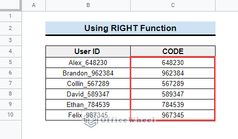
1. Using the RIGHT Function to Get a Substring

Here, if you observe the dataset, each user ID has a unique six-digit code. We will show you how to use the RIGHT function to separate them into another column. Follow the steps to learn how to do this.

📌 Steps:

1. First, select cell B5 and insert the following formula in the formula bar.
2. Next, the formula will return the six-digit code in C5.
3. Then, drag the fill handle to get the rest of the codes.
4. Finally, you will get the result as shown in the image below.

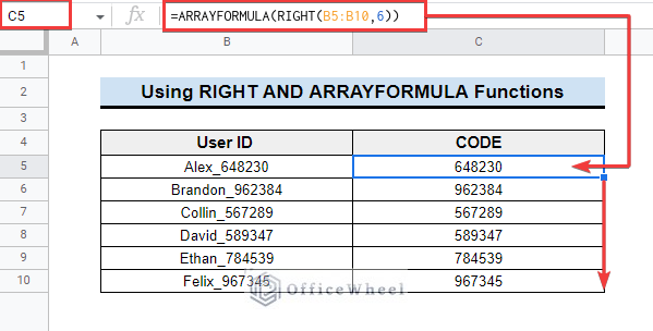
2. Extracting a Substring from Multiple Texts

In this example, we will use ARRAYFORMULA with the RIGHT function. This will allow us to extract substrings from multiple strings at once. The ARRAYFORMULA converts a normal formula into an array formula. This enables the formula to return results from a specific range all at once. Thus, you don’t need to use the fill handle tool as in the previous example.

1. Enter the following formula in cell C5, and you will see all the results at once without having to drag the formula down.

Read more: How to Use ARRAYFORMULA in Google Sheets (6 Examples)

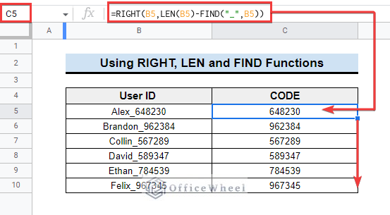
3. Extracting Characters from a String

We can also use the RIGHT, LEN, and FIND functions together to extract a substring from a string. The LEN function returns the length of a string, and the FIND function finds the position of a specific character in a string. We will use these three functions to extract a substring from the string.

Follow the steps below to see how to apply this.

📌 Steps:

1. First, select cell C5 in the given dataset and insert the formula as shown below.
2. Next, drag the fill handle to copy the formula into the cells below.
3. Then, you will get the same results as before.

Read more: How to Remove Characters from a String in Google Sheets (6 Easy Examples)

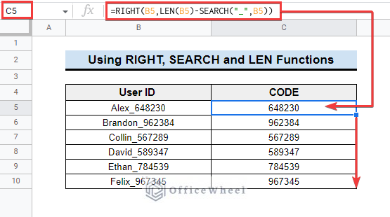
4. Searching and Extracting Characters from Texts

Unlike the FIND function, the SEARCH function is case-insensitive and returns positions of both uppercase and lowercase letters. You can apply this function with the RIGHT function to search for characters and substrings in texts if you need to search for both uppercase and lowercase letters.

The steps are mentioned below.

📌 Steps:

1. First, enter the mentioned formula in cell C5.
2. Next, drag the fill handle down to apply the formula to other cells.
3. This will extract the numbers as illustrated in the following image.

Read more: How to Use the SEARCH Function in Google Sheets (5 Useful Examples)

5. Extracting Values from Character Strings

Although the outputs obtained in the previous methods look like numbers, they are actually in text format. This is because the RIGHT function always returns text outputs. So, you cannot use the outputs as numbers. But you can use the VALUE function to convert these text-like numbers into actual numbers.

1. Apply the following formula in cell C5 and drag the fill handle below to do this.

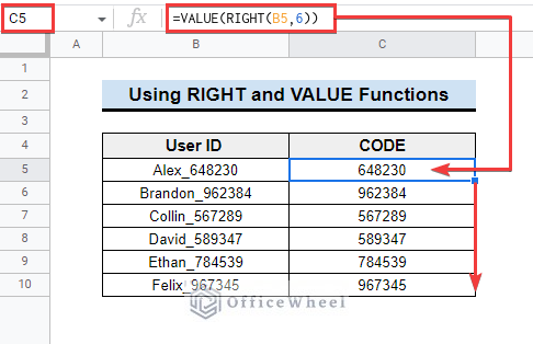
Here, the VALUE function converts text-like numbers into actual numbers.

Read more: How to Convert Text to Date in Google Sheets (3 Easy Methods)

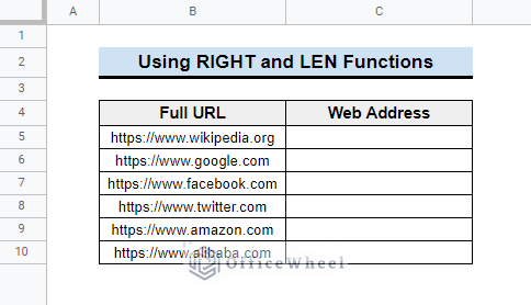
6. Removing Specific Characters from Texts

In this example, we will combine the RIGHT and LEN functions to remove a certain number of characters from the beginning of character strings.

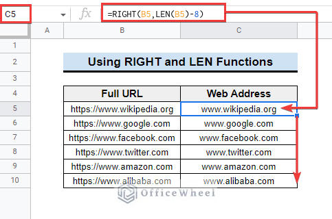
Consider the following dataset containing website addresses with complete URLs. Let’s say you need to remove the “https://” parts from the URLs.

Then, apply the following formula in cell C5 and drag the fill handle below.

Read more: How to Remove the First Character in Google Sheets

What to Do When the RIGHT Function Doesn’t Work in Google Sheets?

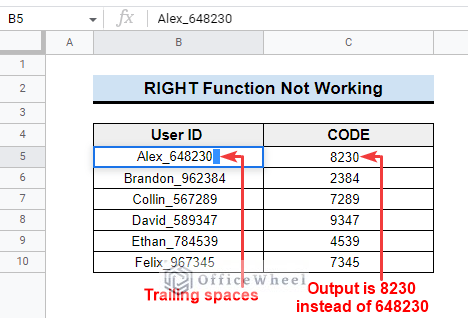
There are a few examples given above to show the various uses of the RIGHT function. However, sometimes the RIGHT function may not work correctly. This usually happens due to extra spaces in the text string.

Consider the following example that uses the RIGHT function. The formula RIGHT(B5, 6) in C5 should return 6 characters from the end. But as we can see, it only returns 4 digits.

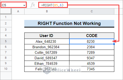
Now, double-click on cell B5, and you will see that there are 2 extra spaces in the string. Since the formula counts them as characters, it seems like the output only contains 4 digits. Remove the spaces, and you will see the correct output.

Read more: How to Use the TRIM Function in Google Sheets (4 Easy Examples)

Points to Remember

• The RIGHT function does not work with dates because the RIGHT function works with strings, and dates are integer numbers.
• The RIGHT function always returns the output as a string. So, if you want to use the output as a number, you need to use the VALUE function as shown in the above example.
• The RIGHT function displays a #VALUE! error if the num_chars argument is negative or less than zero.

Conclusion

We have tried to show you the uses of the RIGHT function in Google Sheets. Hopefully, the above examples will be sufficient for you to understand the applications of the function. Please use the comments section below for any additional questions or suggestions. You can also visit our blog Crawlan.com to learn more about Google Sheets.

Related Articles

• How to Use the SUBSTITUTE Function in Google Sheets (7 Examples)
• How to Use the FIND Function in Google Sheets (5 Useful Examples)
• How to Get Rid of the Dollar Sign in Google Sheets (3 Effective Methods)
• How to Format Date with Formula in Google Sheets (3 Easy Ways)
• How to Use the LEFT Function in Google Sheets (5 Practical Examples)
• Google Sheets: Convert Text to Number (6 Easy Methods)
• How to Fill an Entire Column in Google Sheets (4 Easy Ways)