If you want to copy only the values returned by a formula in a cell, you have to go through the following steps:
- Right-click on the cell containing the formula and select Copy.
- Right-click on the target cell and select Paste special.
- Choose Paste values only from the submenu.
Alternatively, you can also press Ctrl+C to copy and Ctrl+Shift+V to paste only the values. This alternative option is much faster as it utilizes Google Sheets keyboard shortcuts. These shortcuts allow you to perform many manipulations in your spreadsheet without any mouse clicks. Read on to discover these keyboard shortcuts and become a Google Sheets expert!
What are the Keyboard Shortcuts for Google Sheets?
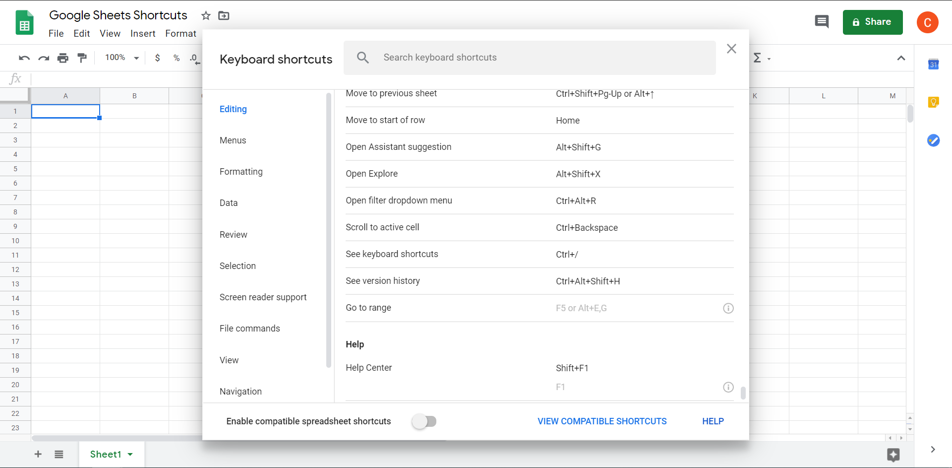
Google Sheets keyboard shortcuts are key combinations on your keyboard that allow you to quickly perform specific tasks in your spreadsheet (navigation, editing, etc.). Everyone knows the basic shortcuts, such as Ctrl+C to copy, Ctrl+V to paste, Ctrl+Z to undo, etc. They also work in Google Sheets. At the same time, there are many other shortcuts that you can explore by pressing Ctrl+/. This is the main shortcut that unveils all the others you can use.
Which Keyboard Shortcuts are Compatible with Spreadsheets and How to Enable Them?
The keyboard shortcuts compatible with spreadsheets are keyboard shortcuts used in another well-known spreadsheet program – Microsoft Excel. If you enable them, you will have 134 additional shortcuts to optimize your workflow.
Please note that the compatible keyboard shortcuts do not work on Mac.
Some of the compatible shortcuts are similar to common shortcuts. For example, to paste values only, you can use the common shortcut Ctrl+Shift+V, as well as the compatible shortcut Alt+H, V, V.
Others are unique. For example, you can paste transpose only with the compatible shortcuts Alt+H, V, T or Alt+E, S, E.
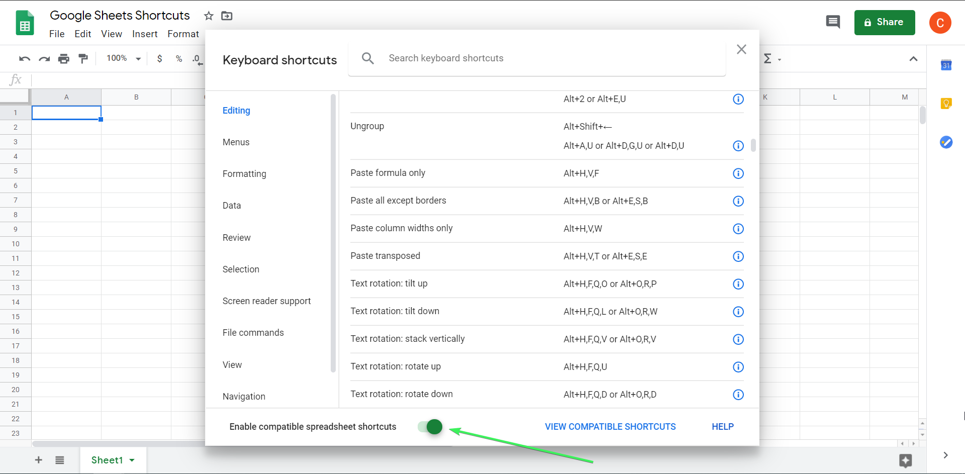
To enable the compatible keyboard shortcuts, press Ctrl+/ and enable them.
Keyboard Shortcuts on PC, Mac, and Chrome OS
To select a column, you need to press Ctrl+Space, and this shortcut works on PC, Mac, and Chrome OS. However, some shortcuts may slightly differ depending on the device you are using.
Mac users usually need to replace the Ctrl key with Command (⌘), and the Alt key with Option (⌥), but this is not the only method. For example, it works for the Insert Time shortcut:
For PC: Ctrl+Shift+;
For Mac: ⌘+Shift+;
But to format as time, you can use the PC shortcut on your Mac without any changes: Ctrl+Shift+2.
Check out this spreadsheet containing a detailed list of keyboard shortcuts for PC, Mac, and Chrome OS in a table.
Keyboard Shortcuts for Android and iPhone/iPad Spreadsheets
If you connect an external keyboard to your Android or iOS device, you can also use a limited number of Google Sheets keyboard shortcuts (the number may depend on the keyboard and language you are using). Check the Google support page for more details.
Google Sheets Keyboard Shortcuts by Category
Now, let’s see what you can do in your spreadsheet without a mouse or trackpad.
Review and Select Commands
| How to | Keyboard Shortcut | Compatible Keyboard Shortcut |
|---|---|---|
Copy and Paste Commands
| How to | Keyboard Shortcut | Compatible Keyboard Shortcut |
|---|---|---|
Editing Commands
| How to | Keyboard Shortcut | Compatible Keyboard Shortcut |
|---|---|---|
Spreadsheet Commands
| How to | Keyboard Shortcut | Compatible Keyboard Shortcut |
|---|---|---|
Menu Access Commands
Please note: Menu access shortcuts only work if compatible keyboard shortcuts are disabled.
| How to | Keyboard Shortcut | Keyboard Shortcut for Mac | Compatible Keyboard Shortcut |
|---|---|---|---|
View Commands
| How to | Keyboard Shortcut | Compatible Keyboard Shortcut |
|---|---|---|
Data Commands
| How to | Keyboard Shortcut | Compatible Keyboard Shortcut |
|---|---|---|
Formatting Commands
| How to | Keyboard Shortcut | Compatible Keyboard Shortcut |
|---|---|---|
Navigation Commands
| How to | Keyboard Shortcut | Compatible Keyboard Shortcut |
|---|---|---|
Number Formatting Shortcuts
| How to | Keyboard Shortcut | Compatible Keyboard Shortcut |
|---|---|---|
File Commands
| How to | Keyboard Shortcut | Compatible Keyboard Shortcut |
|---|---|---|
Function Commands
| How to | Keyboard Shortcut | Compatible Keyboard Shortcut |
|---|---|---|
Grouping Commands
| How to | Keyboard Shortcut |
|---|---|
Screen Reader Shortcuts
| How to | Keyboard Shortcut | Compatible Keyboard Shortcut |
|---|---|---|
Real Use Case: Creating a Sales Dashboard Using Only Keyboard Shortcuts
Now, let’s put your keyboard shortcuts skills into practice. In the blog article “How to Create a Sales Tracker with Google Sheets”, we created an interactive sales dashboard filled with formulas, charts, data validation, and other features. Let’s go through some of those steps again, but with a twist: your mouse will be unplugged or your trackpad will be disabled. You will only be able to use your keyboard to tackle the challenge!
Step 1: Importing Raw Data
The sales dashboard will be powered by data from Pipedrive, so we’ll first import it into Google Sheets. For this, you’ll need to install Coupler.io, a GSheets addon, and set up a Pipedrive importer.
- Open a new spreadsheet – we’re on the spreadsheet containing the descriptions of Google Sheets shortcuts. Create a new one for the sales dashboard.
- Press Ctrl+/ and use Tab to select Enable compatible keyboard shortcuts.
- Once selected, press Space to enable them and Esc to exit the window.
- Now press Alt+F,N, and voila – a new spreadsheet has been created.
Rename the New Spreadsheet
To access menus, we’ll need to disable the compatible keyboard shortcuts for a moment. Press Ctrl+/ and use Tab to select Enable compatible keyboard shortcuts. Once selected, press Space to disable them and Esc to exit the window.
Press Alt+Shift+F to open the File menu and select Rename to specify the name of the new spreadsheet, for example, “Sales Dashboard”.
Install Coupler.io
Coupler.io is a tool that allows you to integrate different applications and data sources into Google Sheets. Check out the available integrations.
Usually, you can install Coupler.io from the G Suite Marketplace via this direct link. But since we’re using only the keyboard, let’s install the addon directly from the spreadsheet.
Press Alt+Shift+N to open the Add-ons menu and select Get add-ons. Use Tab to select the search bar and search for Coupler.io. A few more maneuvers with Tab and Enter, and you’ll see the addon in your spreadsheet (it’s also available in the Add-ons menu).

Friendly note: It’s quite uncomfortable to install addons using only the keyboard, so we recommend doing it with your mouse or trackpad 🙂
Set Up a Pipedrive Importer
We won’t explain how to set up a Pipedrive importer here. The procedure is described in the article “Exporting Data from Pipedrive to Google Sheets”. You can also refer to the knowledge base for more details. The main takeaway is that you need to connect Coupler.io to your Pipedrive account and specify the data entity (Deals, Persons, or Organizations) you want to import. Additionally, you can enable automatic data refresh. This feature imports the data automatically according to a defined schedule!
Use the Tab, Space, and Enter buttons to set up the Pipedrive importer without a mouse or trackpad. It’s not very comfortable, but that’s the challenge!
Launch the importer when you’re ready and welcome your data. For our sales dashboard, we imported Pipedrive Deals.

Step 2: Creating the Sales Dashboard Using Google Sheets Shortcuts
Create a New Sheet for the Dashboard
Now that we have the raw data in our spreadsheet, we can move on to calculations. Let’s enable the compatible keyboard shortcuts (Ctrl+/ => Tab (three times) => Space => Esc) and switch to the sheet where the dashboard will be. Press Ctrl+Shift+PageDown or Ctrl+Shift+PageUp to navigate between your sheets.
Next, press Alt+Shift+S to open the Sheets menu. Choose Rename and type in a name that suits you. We’ve chosen “Dashboard”.
Calculations
We’ll create a table consisting of three columns: Country Name, Conversion Rate, and Total Revenue:
- Country Name – select a cell (A1) and enter the following formula:
= {"Country Name"; UNIQUE(Deals!Z2:Z)}
This will filter all the countries from your Pipedrive deals and automatically attach the name to the column.
- Conversion Rate – select cell B1 and type the column name: “Conversion Rate”. Select cell B2 and apply the following formula:
=COUNTIF(FILTER(Deals!$AL$2:$AL, Deals!$Z$2:$Z=A2), "won")/COUNTA(FILTER(Deals!$AL$2:$AL, Deals!$Z$2:$Z=A2))
Now, select cell B2, hold the Shift key, and select the cells downwards until the end of the country list. Then, press Ctrl+D, and the formulas will be applied to the rest of the countries.
- Total Revenue – perform the same magic for Total Revenue with the following formula:
=SUM(FILTER(Deals!$AF$2:$AF, Deals!$Z$2:$Z=A2, Deals!$AL$2:$AL="won"))
Number Formatting
We want the Conversion Rate to be displayed as a percentage and the Total Revenue to be in US dollars. Here are the shortcuts that can help you:
-
Select cell B2 and press Ctrl+Shift+Arrow down. This will select the data range down to the end. Now, press Ctrl+Shift+5 to apply the Percentage format to the range.
-
Select cell C2 and press Ctrl+Shift+Arrow down to select the data range. Press Alt+O, N, C or Ctrl+Shift+4 to apply the Currency format to the range.
Table Formatting
Now let’s make our table more elegant. Select cell A1 and press Ctrl+Shift+Arrow right to select the cells with the column names. Now, press Ctrl+Shift+B to make them bold.
Press Ctrl+Shift+Arrow down to select the entire table, then press Alt+H, B, A to apply borders.
Inserting a Chart
We’re ready to insert a chart based on our table. For this, select any cell inside the table range and press Ctrl+A to select everything. Then, press Alt+F1 (alternative shortcuts: Alt+N, K or Alt+I, H) to insert a chart. The shortcut worked, and we got the chart, but…
The only way to access the chart editor was by pressing Fn+Menu. However, not all keyboards have this key, and we haven’t found another way to access the chart editor. If you know it, please let us know in the comments.
Conclusion
We took on the challenge and succeeded. Now we know not to dismiss pointing devices (mouse or trackpad) for complex tasks in spreadsheets. Some features, like the chart editor or conditional formatting, are designed for click-based activities. From our experience, editing the chart solely with the keyboard was challenging. As for Google Sheets shortcuts, they can greatly speed up your workflow. However, for that, you need to memorize specific shortcuts so you can apply them when needed. We hope our blog article helps you in this task, and Coupler.io helps you automate data import for your project. Good luck with your data!

