Do you want to have control over the reloading of Importrange data in Google Sheets? If you’re unsure whether it’s possible or not, let me show you a workaround. In this article, I’ll explain a method that allows you to control the reloading of Importrange data from the source file to the destination file in Google Sheets. You can test it yourself to see how effective it is.
Understand Controlling Reloading of Importrange Data
Imagine this scenario: You have given Importrange access to one of your Google Sheets to your employees so they can import certain data from your sheet to theirs. However, you frequently update your sheet based on the progress of the job. Sometimes, you need to incorporate progress updates or rearrange the schedule to focus on the backlogs. In this situation, you don’t want your employees to see the changes you’re making in the background. You want them to only see the old schedule until you push the new data to them. Basically, you want to have a tickbox that controls the reloading of Importrange data in their sheet from your source file.
Let me explain further with an example.
Workaround to Control Reloading of Importrange Data from the Source Sheet
Let’s say you want to import a four-column data from one Google Sheets file to another using the Importrange function. To make it easier to understand, we’ll refer to the files as the ‘Source File’ and the ‘Destination File’. In addition to these files, we’ll also need a ‘bridge’ file. Here’s how the workaround works:
- In the ‘Source File’, you have four tabs – ‘Sch’, ‘New’, ‘Old’, and ‘Control’.
- The ‘Sch’ tab contains the source data that you want to import to the ‘Destination File’. It may be updated frequently.
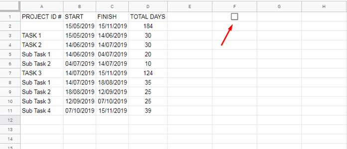
- In the ‘Sch’ tab, there’s a tickbox in cell F1. We’ll explain its purpose later.
- The ‘New’ tab in the ‘Source File’ copies data from the ‘Sch’ tab based on the tickbox in the ‘Sch’ tab. It always has the same data as the ‘Sch’ tab unless you uncheck the tickbox.
- The ‘Old’ tab in the ‘Source File’ contains a backup copy of the ‘Sch’ tab. Before updating the ‘Sch’ tab, you should copy-paste all the values from it (except the tickbox) to the ‘Old’ tab.
- Using the ‘Control’ tab in the ‘Source File’, you can control the reloading of the Importrange data from the source. In other words, you can decide which data to serve to the ‘Destination File’.
Let’s dive into more details.
Source File – Sch, New, Old, and Control Tabs and Their Purpose in Importrange
-
Data in the ‘Sch’ Sheet: This tab contains the source data to import to the ‘Destination File’. It may be updated frequently. There’s a tickbox in cell F1, which we’ll explain later.

-
Data in the ‘New’ Sheet: In cell A1 of this tab, you have a formula that pulls data from the ‘Sch’ tab conditionally. If the tickbox in the ‘Sch’ tab is enabled, the data in the range A1:D will be copied to this tab. Otherwise, the formula will show a custom message.
-
Data in the ‘Old’ Sheet: This tab contains an exact copy or backup of the ‘Sch’ tab.
-
Data in the ‘Control’ Sheet to Control the Reloading of Importrange from the Source File: In this tab, you can control which data (new or old) to push to the ‘Destination File’. There are two tickboxes in cells A1 and A2. Enabling the first tickbox will make the ‘Destination File’ have the data from the ‘New’ tab, while enabling the second tickbox will retain the ‘Old’ tab data. The Vlookup formula in cell B4 of the ‘Control’ tab controls the URL and range used in the Importrange function in the ‘Destination File’.
Changes in File Sharing Settings (Source File)
To make this workaround work, you need to change the file sharing settings of the ‘Source File’ to ‘Private – Only you can access’ or ‘OFF – Specific people’. Then, copy the link.
Mirror File (Bridge) to Control Reloading of Importrange
You’ll need a third file named ‘Mirror File’ as a ‘bridge’ to control the reloading of Importrange. In this file, create a tab named ‘Mirror’ and enter the following formula in the first cell:
=importrange(importrange("Source File URL Here","'Control'!B4"),importrange("Source File URL Here","'Control'!C4"))
Don’t forget to replace ‘Source File URL Here’ with the URL of the ‘Source File’ that you copied earlier.
Changes in File Sharing Settings (Mirror File)
Change the file sharing settings of the ‘Mirror File’ to ‘On – Anyone with the link can view’. Then, copy the link.
Destination File – Importrange Formula that Responds to User Action in the Source
In the ‘Destination File’, enter the following formula in cell A1:
=importrange("Mirror File URL Here","Mirror!A1:D")
Replace ‘Mirror File URL Here’ with the copied link.
Now you have successfully set up the control to reload the Importrange data in Google Sheets! Let me explain how it works:
- When the tickbox in the ‘Sch’ tab is enabled and the first tickbox in the ‘Control’ tab is checked, the ‘Destination File’ will import all the data from the ‘New’ tab.
- When the tickbox in the ‘Sch’ tab is enabled and the second tickbox in the ‘Control’ tab is checked, the ‘Destination File’ will retain the data from the ‘Old’ tab.
- If both tickboxes are enabled or disabled, the ‘Destination File’ will show an error.
- When the tickbox in the ‘Sch’ tab is disabled and the first tickbox in the ‘Control’ tab is checked, the ‘Destination File’ will display a custom message.
That’s how you can control the reloading of Importrange in Google Sheets! Enjoy the enhanced control over your data.
Importrange Resources
If you want to further explore the possibilities of Importrange in Google Sheets, check out these resources:
- How to Freeze Cell in Importrange in Google Sheets
- How to Use IMPORTRANGE Function with Conditions in Google Sheets
- Dynamic Sheet Names in Importrange in Google Sheets
- How to Vlookup Importrange in Google Sheets [Formula Examples]
- How to Use Query With Importrange in Google Sheets
- Importrange Named Ranges in Google Sheets
- Dynamic Column Id in Query Importrange Using Named Ranges
- Relative Cell Reference in Importrange in Sheets
- Dynamic Column in Vlookup Importrange Formula in Google Sheets
- Sumif Importrange in Google Sheets – Examples
- IMPORTRANGE to Import Visible Rows in Google Sheets
Remember, with this workaround, you have the power to control the reloading of Importrange data in Google Sheets. It’s time to take your Google Sheets skills to the next level! Visit Crawlan.com to discover more tips and tricks for enhancing your productivity.


