How to Create a Candlestick Chart in Google Sheets

Did you know that creating a Candlestick Chart in Google Sheets can be quite a challenge? There is not much documentation available on this topic, and even experienced Google Sheets users may face issues with data formatting. But fear not, my friends! In this tutorial, I will show you how to navigate the complexities of creating a Candlestick Chart in Google Sheets and formatting your data for it.

Understanding Candlestick Charts and Stock Value Behavior

Candlestick charts are widely used in the financial world to visualize price movements and changes in stock values. They represent gains and losses through filled and hollow boxes, respectively. But how does this work exactly? Let me explain.

How the Candlestick Chart Reflects Stock Value Behavior

In a Candlestick chart:

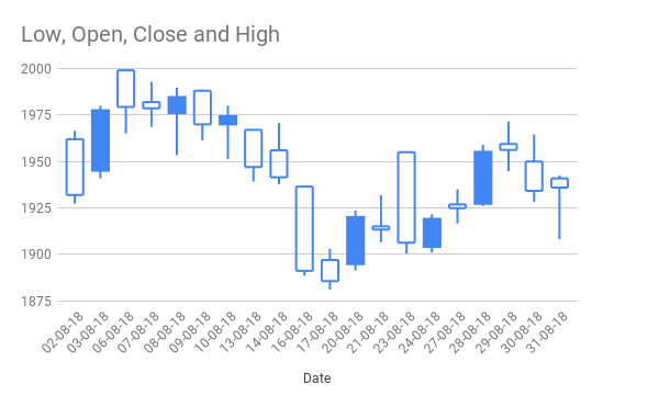
1. Gains are represented by filled boxes when the opening value is less than the closing value.
2. Losses are represented by hollow/empty boxes when the opening value is more than the closing value.

Take a look at the image below to see this in action.

Formatting Data for a Candlestick Chart in Google Sheets

Now that you understand how the Candlestick Chart represents stock values, let’s dive into formatting your data for this chart type. Google Sheets follows a slightly different formatting convention compared to the standard Open-High-Low-Close (OHLC) order. They prefer the Low-Open-Close-High (LOCH) order, and the reason behind this remains a mystery.

Formatting Data in the LOCH Format

To format your data for a Candlestick Chart in the LOCH format, follow these steps:

1. Manually enter your data in the correct format, as shown in the example above. In this example, the source data is in the range A5:E8.
2. If you’re using the GoogleFinance function to populate historical stock prices for your chart, you will encounter one issue. The data generated by the GoogleFinance function will be in the OHLC format. But don’t worry, you can use the Query function to convert this data to the LOCH format.

Plotting a Candlestick Chart Using GoogleFinance Historical Stock Price Data

Let’s now explore how to plot a Candlestick Chart in Google Sheets using GoogleFinance historical stock price data. Follow these steps:

1. Use the following GoogleFinance formula to populate the historical price of your chosen stock (in this case, HDFC from NSE India):

   =GOOGLEFINANCE("symbol"; "all"; "start_date"; "end_date")

2. Modify the formula to suit your needs. For example:

   =GOOGLEFINANCE("NSE:HDFC", "all", "01/08/2018", "31/08/2018")

3. The default column order generated by the GoogleFinance function may not be suitable for plotting a Candlestick Graph. You need to rearrange the columns and format the first column to text.
4. Use the Query function to format the OHLC data to the LOCH format. Here’s an example of the modified formula:

   ={ArrayFormula(text({"Date"; int(query(query(googlefinance("NSE:HDFC", "all", "01/08/2018", "31/08/2018"), "Select Col1", 1), "offset 1", 0))}, "DD-MM-YY")), query(googlefinance("NSE:HDFC", "all", "01/08/2018", "31/08/2018"), "Select Col4,Col2,Col5,Col3", 1))}

5. Once you have properly formatted your data, select the range A1:E (considering the above Query formula in A1). Then go to the menu Insert > Chart and choose Candlestick Chart.
6. Voila! Your finished Candlestick chart will look something like this:

Conclusion

Congratulations, my dear friends! You now have the knowledge and skills to create Candlestick charts in Google Sheets. If you encounter any difficulties with the data formatting process using Query, feel free to reach out to me for assistance. And if you found this tutorial helpful, don’t forget to share it on social media and leave a comment below. Keep shining bright! Crawlan.com