Learn the tricks to easily filter your data by month using the filter menu in Google Sheets. Filtering a dataset in Google Sheets can be done in two ways: using the Filter Menu command or using the Filter Functions.
Filter Functions: The Handy Tool You Need!
Yes, there are filter functions in Google Sheets! These functions, namely Filter and Query, are incredibly handy when it comes to filtering data. Personally, I prefer using the Query function because I am more familiar with it. However, there are times when we can’t solely rely on functions to filter data.
The functions in Google Sheets extract the filtered data and place it in a new range. If you’re someone who doesn’t want that, then the Filter Menu in Google Sheets is the perfect solution for you.
The Flexibility of the Filter Menu
The Filter Menu in Google Sheets not only allows you to filter your data but also gives you the flexibility to apply custom formulas similar to conditional formatting rules. This means you can customize your filters to your heart’s content.
In this Google Sheets tutorial, I will show you a custom formula that you can use in the Filter function’s custom formula field to filter your data by month. But first, let me clarify what exactly I mean by “filter by month.”
Filtering a Column Between Two Given Months
Filtering a column between two given months is the process of selecting data that falls within a specific range of months. If you’re interested in grouping your data month-wise, I have the perfect example for you, which you can find on Crawlan.com.
Now, let’s proceed to the main topic. Here is the custom formula you can use to filter your data by month in the Filter Menu in Google Sheets.
Custom Formula to Filter by Month Using the Filter Menu in Google Sheets
Sample Data:
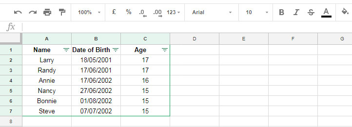
To filter column B for the months between June and July, follow these steps:
Steps to Filter by Month Using the Filter Menu in Google Sheets:
- Select the data range you want to filter, for example, A1:C7.
- Go to the “Data” menu and select “Filter,” then click on “Create a filter.”
- Click on the field label “Date of Birth.” In the dropdown menu, select “Filter by condition,” and under “Custom formula is,” apply the following custom formula.
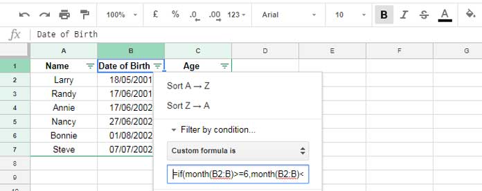
Formula:
=if(month(B2:B)>=6, month(B2:B)<=7)That’s it! By using this custom formula, you can easily filter the dates in column B between June 1st, 2018, and July 31st, 2018. In other words, this custom formula filters the months of June and July.
Feel free to modify the month numbers in the formula to filter any desired range of months.
If you prefer filtering column B using a formula in a new range, here is the Filter formula for you:
=filter(A2:C, month(B2:B)>=6, month(B2:B)<=7)For more information on filtering in Google Sheets, check out these related articles:


