Are you a beginner working with Google Docs Spreadsheets? If so, I have a valuable time-saving tip for you! In this article, we’ll explore a unique approach to filtering data in Google Sheets. Unlike the QUERY function, which doesn’t retain hyperlinks, we’ll use the FILTER function to efficiently filter data and transfer it to different sheets within the same workbook.
Filtering Data to Separate Sheets: Can It Be Done in Excel Too?
In Microsoft Excel, you can filter data to separate sheets or ranges using the advanced filter option. However, there’s a distinction with the FILTER function in Google Sheets.
The FILTER function in Google Sheets not only copies the filtered data but also retains any hyperlinks. This means that any changes made to your master data will be reflected in the filtered data, ensuring that your hyperlinks remain intact.
Update: The FILTER function is now available in Excel as well (not in all versions), though the usage might be slightly different.
Tips for Transferring Filtered Data with Links to Different Sheets or Sheet Tabs
To achieve this, we will use the FILTER function in Google Docs Spreadsheet. The syntax is as follows:
Syntax:
FILTER(range, condition1, [condition2, ...])
The entire process is straightforward if you follow the step-by-step tutorial below. Just refer to the example provided to master the FILTER function and apply it later as needed.
Steps
Step 1:
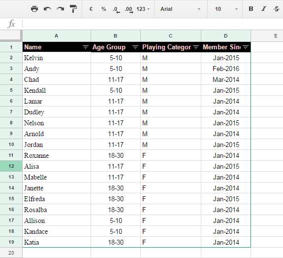
Enter the provided sample data in a new Google Sheets spreadsheet or copy the sample sheet by clicking the button immediately after the image.
Sample Sheet
Observe that the data represents a list of club members and their corresponding age groups.
Step 2:
Create three new tabs or sheets and name them as follows: ‘Age Group 5-10,’ ‘Age Group 11-17,’ and ‘Age Group 18-30.’
Step 3:
Copy the column header to the first row of each of the newly created sheets.
Step 4:
Apply the FILTER function to the second cell of each new tab, i.e., cell A2.
The formula for the first tab is:
=FILTER('Master Folder'!A1:D19,'Master Folder'!B1:B19="5-10")Please refer to the syntax given above. The formula selects the range and provides the filter criteria.
Similarly, the formula for the second tab is:
=FILTER('Master Folder'!A1:D19, 'Master Folder'!B1:B19="11-17")And the formula for the third tab is:
=FILTER('Master Folder'!A1:D19, 'Master Folder'!B1:B19="18-30")This will generate the filtered data in the respective sheets automatically. That’s it!
Conclusion
By following these steps, you now have a total of four sheets. The first sheet contains the master dataset, while the other three sheets contain the filtered data. Remember to update the cell reference in the formula for each sheet if you add or delete rows in your master data. Alternatively, you can use open-ended ranges such as A1:D and B1:B instead of A1:D19 and B1:B19.
If the sample data contains hyperlinks, the FILTER function will transfer them along with the filtered data. Simply hover your mouse pointer over the text to see the clickable links.
And here’s the best part – if you add or delete data in the source sheet, the filtered data in separate sheets will automatically refresh!
For more advanced filtering techniques, check out the tutorials available on our website, Crawlan.com.
Happy filtering!


