Are you using Google Sheets and wondering how to filter the top 3 most frequent strings? Look no further! In this article, I’ll walk you through step by step on how to achieve this. It’s a handy trick that can save you time and effort when working with large datasets. So let’s dive in!
The Problem with the Formula
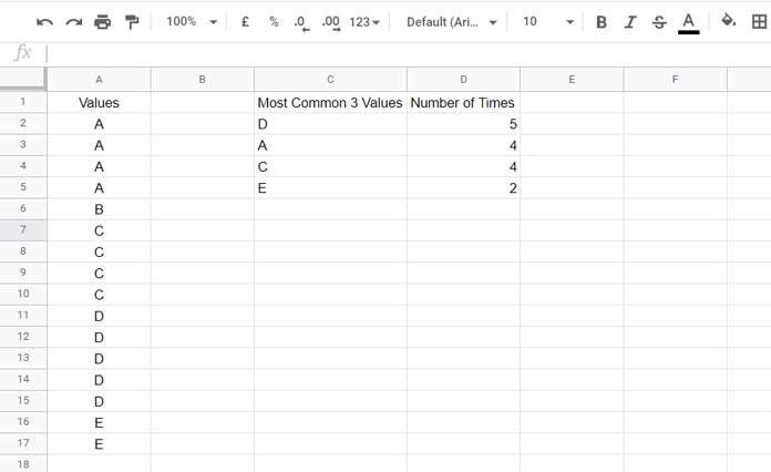
Before we get started, let’s address an important point about the result that the formula will return. Let’s say we have five strings with different occurrences. The formula will return four strings instead of the desired three. Why? Well, this is because two strings, A and C, are tied for the second position with four occurrences each. Don’t worry, though, we’ll show you how to filter out the top three strings.
Example
To illustrate this process, let’s consider the following example. In a Google Sheet, we have a list of texts in column A. We want to find the top three most frequent strings and their respective occurrences. In cell C2, you can use the provided formula to achieve this. As you can see in image #1, the formula returns four values due to the tie between strings A and C.
Filtering the Top 3 Most Frequent Strings in Google Sheets
Now, let’s move on to the steps involved in filtering the top three most frequent strings in Google Sheets. We’ll be using a few helper columns initially, but don’t worry, we’ll remove them later.
Step #1 – COUNTIF Array to Return the Count of Strings
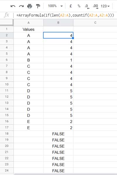
In this step, we’ll use a COUNTIF array formula to find the count of each string in column A. To do this, enter the following formula in cell B2:
=ArrayFormula(if(len(A2:A),countif(A2:A,A2:A)))The COUNTIF function will return how many times each string occurs. You can see the result in image #2.
Step #2 – Find the Number of Times the Most Frequent N Strings Occur
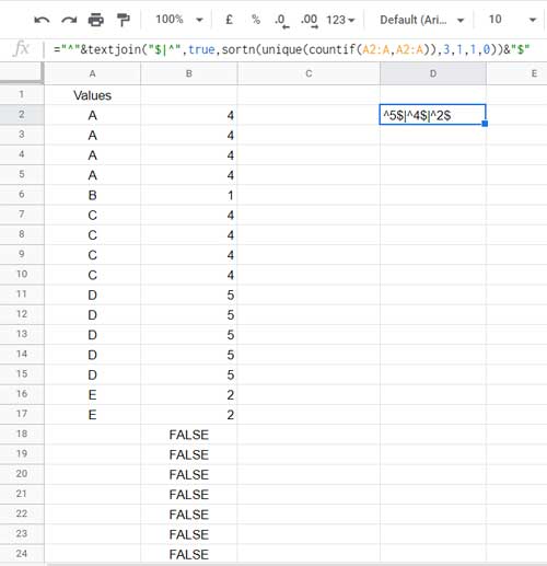
In the next two steps, we’ll determine the number of most frequent strings to filter. In cell D2, enter the following formula:
=sortn(unique(countif(A2:A,A2:A)),3,0,1,0)The above formula will return the top three values after sorting them in descending order. If you want to filter the top five most frequent strings, simply change the number 3 to 5 in the formula. For a detailed explanation of the formula, refer to image #3.
Step #3 – Filter the Most Frequent 3 Strings Using Number of Times
Now comes the final step. In cell C2, enter the following formula:
=unique(filter({A2:A,if(len(A2:A),countif(A2:A,A2:A))},regexmatch(if(len(A2:A),countif(A2:A,A2:A))&"","^"&textjoin("$|^",true,sortn(unique(countif(A2:A,A2:A)),3,1,1,0))&"$")))This formula will filter the most frequent three strings based on the number of times they occur. It will remove any duplicates and sort the second column in descending order.
And just like that, you’ve successfully filtered the top three most frequent strings in Google Sheets! Say goodbye to manual sorting and save valuable time on data analysis.
For more advanced usage or to filter a different number of strings, feel free to tweak the formula as needed. It’s a versatile method that can be adapted to suit your specific needs.
I hope this article has been helpful to you. If you’d like to explore more tips and tricks related to Google Sheets, visit Crawlan.com for more valuable insights. Happy filtering!


