Have you ever wondered if it’s possible to highlight all the cells with formulas in Google Sheets? Well, guess what? It is possible! Many Google Spreadsheet users may think otherwise because they believe there is no alternative to Excel’s “Go To” Command in Google Doc Spreadsheets. But fear not, my friends, for I am about to reveal the secret to highlighting those formula-filled cells!
The Power of Conditional Formatting
In Excel, highlighting cells with formulas is a breeze with the “Go To” command (Ctrl+G) Special. This command temporarily highlights cells that contain formulas. However, in Google Sheets, we can achieve the same result using Conditional Formatting, which is just as powerful, if not more.
Utilizing the ISFORMULA Function
To highlight cells with formulas in Google Sheets, we will harness the power of the ISFORMULA function. This magical function allows us to test any cell for a formula and return either TRUE or FALSE. By using a custom formula with Conditional Formatting, we can achieve our goal of highlighting those formula cells.
Below is an example of how you can use the ISFORMULA function in Conditional Formatting to find all the cells containing formulas:

Tips to Highlight All the Cells with Formulas
Now, it’s time to unveil the step-by-step process to highlight all those hidden formula cells in Google Sheets:
- Start by navigating to cell A1.
- Go to the “Format” menu and select “Conditional Formatting.”
- Refer to the image below to set the necessary rules for Conditional Formatting.
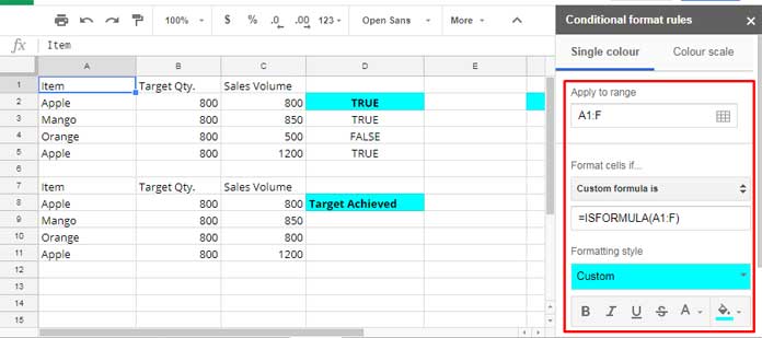
- Adjust the “Apply to Range” based on your spreadsheet’s needs. For example, if your sheet has cells up to column F, you can set the range as A1:F.
- Choose whether to apply this conditional formatting rule to the selected range or the entire sheet.
- From the drop-down menu, select “Custom formula is” and enter the custom formula as shown above. Make sure to adjust the formula range based on your “Apply to range” selection.
- Finally, select a formatting style, and voila! All the cells with formulas will be magically highlighted.
Now you know how to easily highlight all the cells with formulas in Google Sheets using Conditional Formatting. But what if you want to find those formula cells without using Conditional Formatting? Fear not, for I have an answer for that too!
Finding All the Cells Containing Formulas – No Conditional Formatting Required
If you prefer to view all the cells containing formulas without utilizing Conditional Formatting, there are two methods you can try:
- Use the shortcut key “Ctrl+~” to instantly reveal all the formulas in your sheet.
- Alternatively, you can go to the “View” menu and choose “Show Formulas” to display all the formulas right before your eyes.
And there you have it, my dear friends! You now possess the knowledge to easily highlight all the cells with formulas in Google Sheets, whether through the power of Conditional Formatting or by simply revealing the formulas themselves. Go forth and conquer your spreadsheets with confidence!
That’s all for now. Enjoy. And don’t forget to check out Crawlan.com for more exciting Google Sheets tips and tricks!
This article is brought to you by Crawlan, your go-to source for all things Google Sheets.


