How to Partially Flatten a Multi-Column Array in Google Sheets

You might find yourself in a bind when you need to partially flatten a multi-column array in Google Sheets. Flattening refers to condensing values from one or more arrays into a single column. It’s different from using TRANSPOSE, which changes the orientation of one or more arrays. Let me explain further with an example.

Imagine you have data in four columns on a sheet, structured like this: the first column contains descriptions of construction activities (tasks), while the next three columns represent the completion weightage for each activity in different weeks. Your goal is to partially flatten this multi-column array using the FLATTEN function in Google Sheets. In other words, you want to combine the last three columns (task weightage) and align them properly with the values in the first column (tasks). The desired result is a final output consisting of two columns: activities and weightage.

Typically, attempting this method will be unsuccessful. For instance, when you try “=FLATTEN(B3:D8)” in cell G2, you’ll notice that the partially flattened range/array (B3:D8) is misaligned with the values in the range A3:A8. Obviously, this won’t work. To overcome this issue, you need to insert two blank cells between each activity in the range F2:F7 to make the partially flattened data align correctly.

Partially Flattening a Multi-Column Array into Two Columns

To partially flatten a multi-column array in Google Sheets, I’ve used the following two formulas (refer to range I2:J19):

In cell I2:

=ArrayFormula(flatten({A3:A8,iferror(A3:B8/0)}))

In cell J2:

=flatten(B3:D8)

Let me break it down for you.

Note: You can combine the I2 and J2 formulas and use them as a single formula in I2. However, I don’t recommend this approach as it may cause issues when you want to keep more than one column untouched.

Formula Explanation

First, let’s dive into the I2 formula, which inserts blank cells between tasks. Our objective is to return two blank cells below each activity (task). How can we achieve that? By flattening one value column and two blank columns.

The generic formula is:

=flatten(1_value_column, 2_blank_columns)

1_value_column: A3:A8
2_blank_columns: iferror(A3:B8/0)

To create two virtual blank columns, we use IFERROR as shown above. Additionally, we wrap the FLATTEN function with ArrayFormula because IFERROR is a non-array function. That’s how we solve the problem!

This methodology allows us to partially flatten a multi-column array in Google Sheets.

Note:
Let’s assume you have infinite column arrays, such as A3:A and A3:B in the I2 formula and B3:D in the J2 formula. In that case, you can use FILTER with the formulas as follows:

In cell I2:

=flatten({filter(A3:A,A3:A<>""),
          filter(iferror(A3:B/0),A3:A<>"")})

In cell J2:

=flatten(filter(B3:D,A3:A<>""))

Partially Flattening a Multi-Column Array into Three Columns

Now, let’s consider a scenario where you want to insert one more column between columns A and B to represent the total weightage of each activity in the above construction schedule (range A2:D8). Here’s the modified data:

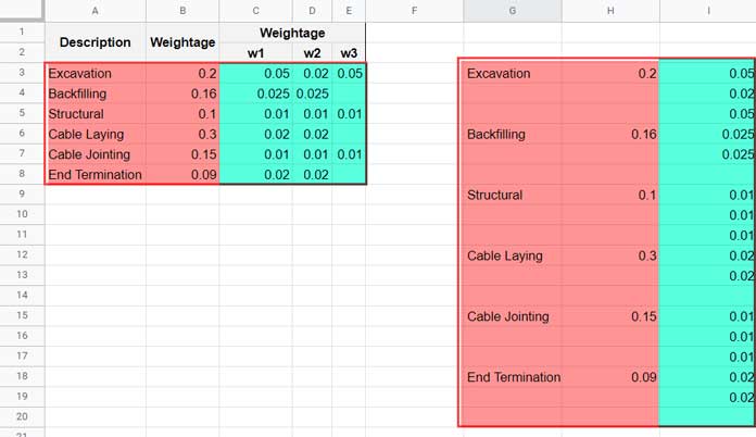
Partially Flatten a Multi-Column Array - Example 2

To partially flatten a multi-column array into three columns, you can use the same formulas mentioned above with some slight modifications. Use formula I3 to flatten range C3:E8 directly and insert blank cells in range A3:A8 in formula G3.

In cell G3:

=ArrayFormula(flatten({A3:A8,iferror(A3:B8/0)}))

In cell I3:

=flatten(C3:E8)

But wait, we still need to insert blank cells between the weightage values in range B3:B8 and display them in range H3:H20. The following formula accomplishes that:

In cell H3:

=ArrayFormula(flatten({B3:B8,iferror(A3:B8/0)}))

Additional Tips for More than Three Columns

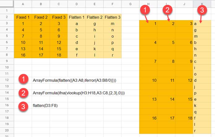
If you have several columns to keep on the left side of the data, I suggest using a Vlookup Array Formula. Here’s how it works:

In this example, you can replace the formula in cell H3 with the following:

=ArrayFormula(ifna(vlookup(G3:G18,A3:B8,{2},0)))

The VLOOKUP function searches for tasks in range G3:G18 within range A3:B8 and returns the total weightage from range B3:B8.

What makes this formula useful? By changing {2} to {2,3}, you can return values from two columns simultaneously. Take a look at the screenshot below for a self-explanatory example:

4-column output - example