Google Sheets offers a variety of formula options to retrieve the column header of the minimum value in a row. In this article, we will explore three of the best formulas: a non-array formula (Filter), and two array formulas (Vlookup and Lambda). Each formula works differently and has its advantages.
Formula to Return the Column Header of Min Value in Google Sheets
Imagine you have a team of five employees, and you want to assess their daily sales to identify the underperforming employee each day. You have a table with the employee names in the header row and their corresponding daily sales in the following columns.
We can use the Filter formula to achieve this. Assuming your table is in the range A1:F10, you can enter the following Filter formula in cell H2 and drag it down to retrieve the column header of the minimum value in each row:
=ifna(filter($B$1:$F$1, B2:F2=minifs(B2:F2,B2:F2,">0"), B2:F2<>""))
This formula uses the MINIFS function to find the minimum sales quantity in each row, excluding zero and blanks. The FILTER formula then filters the column headers (employee names) that match the MINIFS result. If a row is blank or contains only zeros, the MINIFS function will return zero. In such cases, the formula uses the condition B2:F2<>””, which returns #N/A. The IFNA function is used to remove this error. When you drag the formula down, it applies to other rows.
If you’re curious about how this formula works in action, check out this example live (GIF) here.
Array Formula 1 to Retrieve the Column Header of Min Value – VLOOKUP
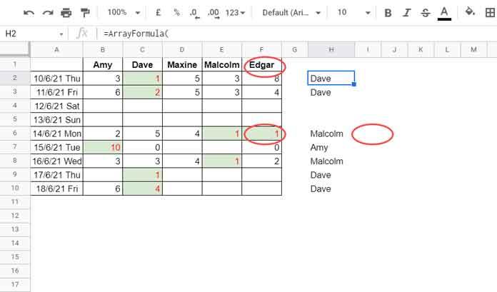
You can also use an array formula with Vlookup to retrieve the column header of the minimum values in Google Sheets. While this formula works, it has a drawback. In the previous example, the Filter formula returned “Malcolm” and “Edgar” as the minimum values in row #6. However, this array formula would only return the first minimum header, which is “Malcolm”.
=ArrayFormula(ifna(if(len(A2:A), vlookup(row(A2:A)&"~"&dmin(transpose(if(A2:F>0,A2:F,)), sequence(rows(A2:A),1), {if(,,);if(,,)}), Query(split(flatten(row(A2:A)&"~"&if(B2:F>0,B2:F,)&"🐟"&B1:F1),"🐟"), "Select * where Col1 is not null and Col2 is not null"),2,0))))
If you prefer using this array formula to retrieve the column header of the minimum value in each row, let’s break down how it works:
- The SEARCH_KEY is the combination of row numbers and minimum values in each row.
- The RANGE is the unpivoted data from columns B to F.
- The formula uses the VLOOKUP function to retrieve the column header of the minimum value in each row, excluding zero.
- Please note that if there are multiple minimum values in a row, this array formula will only return the first occurrence from left to right.
To see this array formula in action, refer to the following image:
Array Formula 2 to Retrieve the Column Header of Min Value – LAMBDA
In recent updates, Google Sheets introduced the capability to expand non-array formulas using LAMBDA helper functions (LHF). We can use the BYROW LHF to expand our first filter-based non-array formula and retrieve the column header of the minimum value in each row.
=byrow(B2:F,lambda(r, join(", ",ifna(filter($B$1:$F$1,r=minifs(r,r,">0"),r<>"")))))
This formula combines column names (headers) if there are multiple occurrences of the minimum values. Unlike the non-array formula, which returns “Malcolm” and “Edgar” in two separate cells (row #6), the Lambda formula will JOIN them.
That’s all for now! Enjoy exploring these formulas to retrieve the column header of the minimum value in Google Sheets. If you’re interested, you can also check out the related article on finding the column header of the maximum value using an array formula.


