How to Sort Pivot Table Grand Total Columns in Google Sheets

The Pivot table is a powerful tool for summarizing and reorganizing data in Google Sheets. It’s also widely used in other spreadsheet applications. At some point, you may find yourself wanting to sort the Grand Total columns at the bottom of the Pivot table report. Luckily, sorting these columns in Google Sheets is easy and straightforward. In this tutorial, I will show you how to do it step by step.

Sorting Grand Total Columns in Descending or Ascending Order

To sort the Grand Total columns in a Pivot table, you need to make some changes in the “Columns” field of the Pivot table editor. If the editor is currently closed, hover your mouse pointer over the Pivot table report, and you’ll see a pencil/pen icon at the bottom left corner. Click on it to open the editor panel.

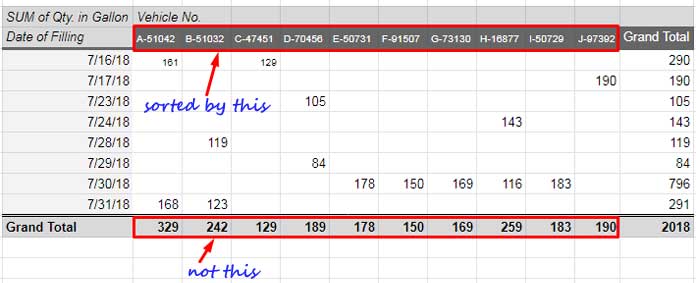
Inside the Pivot table editor, locate the “Columns” field. By default, it is sorted in ascending order based on the field labels. To change the sorting order, select the field used in the “Values” section (with the aggregation SUM) and then choose “Grand Total.”

By changing the sorting from “Ascending” to “Descending,” you can modify the sort order of the Pivot table Grand Total columns. It’s as simple as that!

Steps to Sort Pivot Table Grand Total Columns

Before we dive into sorting the Grand Total columns, let me guide you through creating a Pivot report without sorting. This will help you better understand the process. Follow these steps:

1. Select the data range you want to use for the Pivot table (for example, A2:C16).
2. Go to the menu, click on “Insert,” and then select “Pivot table.”
3. Choose whether you want to create the Pivot table on a new sheet or an existing sheet.
4. Inside the Pivot table editor panel, you need to add three components: Rows, Columns, and Values.

In our data example, we have three columns. Here’s how to include them in the Pivot table:

• Values: Add the column containing the values you want to sum (for example, column B – “Qty. in Gallon”). Select the appropriate aggregation function from the drop-down menu (e.g., SUM).
• Rows: Include the data in the column you want to use for the rows (e.g., column A – “Date of Filling”).
• Columns: Add the column you want to use for the columns (e.g., column C – “Vehicle No.”).

Once you’ve set up the Pivot table, you’ll notice that the columns are sorted by default based on the field labels (in this case, “Vehicle No.”). Feel free to check the report to see the initial sorting.

That’s it for creating the Pivot report without sorting. Now, let’s move on to sorting the Grand Total columns.

Additional Resources

If you want to further enhance your Pivot table skills, here are some additional resources you may find helpful:

1. How to Use GETPIVOTDATA Function in Google Sheets
2. Create an Age Analysis Report Using Google Sheet Pivot Table
3. Month Wise Pivot Table Report in Google Sheets Using Date Column
4. Group Dates in Pivot Table in Google Sheets (Month, Quarter, and Year)
5. Adding Calculated Field in Pivot Table in Google Sheets
6. Drill Down in Pivot Table in Google Sheets (Date Field)

I hope this tutorial has been helpful in guiding you through the process of sorting Grand Total columns in a Pivot table in Google Sheets. Remember, the Pivot table is a versatile tool that can greatly assist you in analyzing and presenting data effectively. Enjoy exploring its features and functionalities!

That’s all for now. If you have any questions or need further assistance, don’t hesitate to reach out. Happy sorting!