Have you ever struggled with sorting pivot table rows in Google Sheets? Maybe you wanted to sort them by a specific column other than the first one, but couldn’t find a built-in option to do so. Well, fear not! I have a workaround that will solve your problem and allow you to sort pivot table rows by any column you desire.
The Issue
By default, Google Sheets only provides the option to sort pivot table rows by the first column. This can be frustrating if you want to sort them by a different column, such as “P.O. Date.” The sorting order would be based on the following sequence: Item/SUM of Order Qty -> Supplier/SUM of Order Qty -> P.O. Date/SUM of Order Qty. As you can see, the desired sorting is not achieved.
The Solution
To sort pivot table rows by a specific column, we need to use a helper column and an array formula. Let me guide you through the process.
Step 1: Prepare the Data
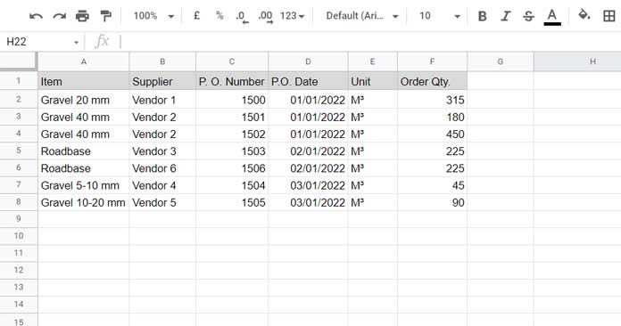
First, make sure you have the necessary data in your Google Sheets. For this example, let’s assume we have a mockup purchase order details table with six columns: “Item,” “Supplier,” “P.O. Date,” “SUM of Order Qty,” and two additional columns for the helper column. You can find the sample data here.
Step 2: Set Up the Pivot Table
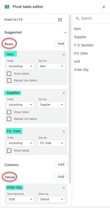
Now, let’s create a pivot table based on the data. Drag and drop the first three fields (Item, Supplier, P.O. Date) under the “Rows” section in the pivot table editor. Then, drag and drop the “Order Qty” field under the “Values” section. Refer to the screenshot here for the exact settings.
Step 3: Add the Helper Column
To sort the pivot table rows by the desired column, we need to add a helper column. In this case, we’ll use column G. Apply the following array formula in cell G1 to sort the P.O. Date column in ascending order:
=ArrayFormula(ifna({"Helper";rank(D2:D,D2:D,1)}))If you want to sort the column in descending order, use the following formula instead:
=ArrayFormula(ifna({"Helper";rank(D2:D,D2:D,0)}))Step 4: Adjust the Pivot Table
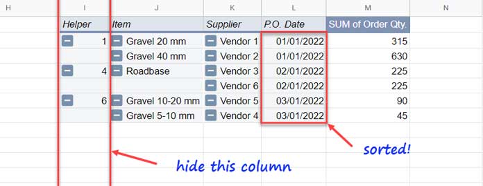
Now, go back to the pivot table editor and drag the new “Helper” field above the “Item” field. This change will ensure that the pivot table rows are sorted based on the values in the helper column. Lastly, you can hide the helper column within the pivot table report to keep it clean.
And there you have it! Your pivot table rows are now sorted by the desired column, not by the first one. Take a look at the final result here.
Conclusion
Sorting pivot table rows by a specific column in Google Sheets may require a workaround, but it’s definitely achievable. By adding a helper column and using an array formula, you can sort the rows based on any column you want. Remember to adjust the pivot table settings accordingly and hide the helper column for a polished look.
For more tips and tricks on Google Sheets and other spreadsheet-related topics, visit Crawlan.com. Happy sorting!

