Another juicy logical sum tutorial coming your way! If you’ve ever wondered how to use SUMIF when multiple criteria are in the same column in Google Sheets, you’re in luck. Buckle up and follow this step-by-step tutorial to become a pro at summing with multiple criteria.
There are plenty of SUMIF formula tutorials out there, but let’s dive right into this one. The traditional approach would be to use one SUMIF formula for each criterion and then add them together like this:
SUMIF(range, criterion, sum_range) + SUMIF(range, criterion, sum_range)No doubt, it gets the job done. However, I’m here to introduce you to a 100% better solution. There is an alternative way to SUMIF when multiple criteria are in the same column using Google Sheets. Exciting, right?
The Normal Way: SUMIF When Multiple Criteria in One Column
Let’s start by understanding the normal way of using SUMIF with multiple criteria in the same column. Take a look at the example below:
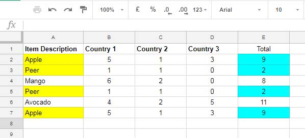
In this example, we want to calculate the sum of the fruits “Apple” and “Pear.” The criteria are highlighted in yellow in Column A, and the totals are highlighted in cyan in Column E. Traditionally, we would use two individual SUMIF formulas:
=SUMIF(A2:A7, "Apple", E2:E7) + SUMIF(A2:A7, "Pear", E2:E7)And voila, the result is 22. But wait, there’s a better way!
The Array-Based Solution: SUMIF When Multiple Criteria in the Same Column
Drumroll, please! Introducing the recommended SUMIF formula in this case:
=SUM(ArrayFormula(SUMIF(A2:A7, {"Apple";"Pear"}, E2:E7)))Yes, you heard it right. We can include both criteria in one single SUMIF formula using curly brackets. To make it even more powerful, we use the ArrayFormula and SUM functions.
With this formula, you can easily sum values that meet multiple criteria in the same column in Google Sheets. But here’s a friendly pro tip: If you omit the SUM function in this formula, you’ll get the total of the fruits “Apple” and “Pear” in separate cells. Handy, isn’t it?
Generate Group-Wise Summary Using SUMIF in Google Sheets
But wait, there’s more! You can take this array-based SUMIF formula a step further and create a group-wise summary of fruit items. Check out the image below for a visual representation:
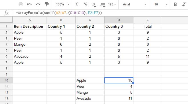
In this example, I’ve applied the UNIQUE formula in cell C10 to extract the unique fruit names from column A. Then, in cell D10, I’ve used the following SUMIF formula to calculate the total of each fruit item:
=ArrayFormula(SUMIF(A2:A7, {C10:C13}, E2:E7))But hold on, there’s an even more advanced technique for the daring ones out there!
For Advanced Users: A Shorter Grouping Formula
If you’re looking to streamline your grouping, you can combine the UNIQUE and SUMIF functions into one formula, like so:
={UNIQUE(A2:A7),ArrayFormula(SUMIF(A2:A7, {UNIQUE(A2:A7)}, E2:E7))}Simply replace the cell references with the formulas that return the unique values. In this case, the formulas return the values in cell C10:C13. Trust me, it will save you time and make you feel like a Google Sheets wizard!
Now that you have all these fantastic formulas at your disposal, it’s time to put them to the test. Apply them one by one in your own Google Sheets and see how they work their magic. Happy summing!
Remember, for more exciting tips and tricks, head over to Crawlan.com. Stay tuned for more Google Sheets goodness!


