How to Use ISNUMBER Formula in Google Sheets: Unleashing Its Practical Applications

You may think that the ISNUMBER formula in Google Sheets is simple and straightforward. But hold on! Let me show you how this seemingly basic function can actually be a hidden gem in certain situations. In this tutorial, we will not only explore how to use the ISNUMBER formula in Google Sheets but also discover its practical applications.

Syntax: ISNUMBER(value)

The ISNUMBER function is designed to check whether a value is a number. If it is indeed a number, the function returns TRUE; otherwise, it returns FALSE.

Practical Use of ISNUMBER Formula in Google Sheets

Let’s first understand the regular use of the ISNUMBER function:

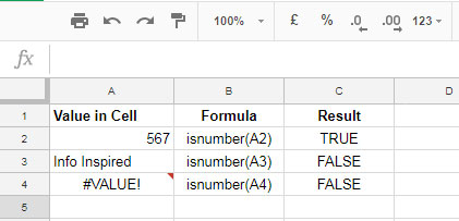
In the above examples, only the value in Cell A1 is considered a number, so the ISNUMBER function returns TRUE. Now, take note of the following two variations of the ISNUMBER formula:

= --isnumber(A2)
=isnumber(A2)*1

Either of the above variations can return 1 instead of TRUE. If the ISNUMBER function returns FALSE, these variations would return 0.

But why are these variations relevant here? Let me illustrate this with a practical example using the ISNUMBER function in Google Sheets.

In the screenshot below, we have a FIND formula. This formula is case-sensitive and works similarly to the Google Sheets EXACT function. It helps to match two cells for identical or case-sensitive texts.

If there is a match, the FIND formula returns 1; otherwise, it returns #VALUE!. On the other hand, the EXACT function returns TRUE or FALSE.

So, what’s the point? Here’s the catch: ISNUMBER combined with FIND can act as an EXACT function. This means that the following formula would return FALSE instead of #VALUE!:

=isnumber(find(A1,B1))

Similarly, the following variation can return 1 or 0:

=isnumber(find(A1,B1))*1

Why is this important? Well, you can use this combination as an alternative to the EXACT function in Google Sheets.

Array functions typically do not accept the EXACT function. In such cases, you can use the ISNUMBER_FIND combo or even FIND alone for an exact match. If you’re interested in learning more about case-sensitive SUMIF, check out our tutorial on our website.

Furthermore, I have utilized the ISNUMBER_FIND combo for a case-sensitive COUNTIF operation in Google Sheets.

Other Uses of ISNUMBER

The ISNUMBER function is also handy when used in combination with an IF logical test. Let me explain:

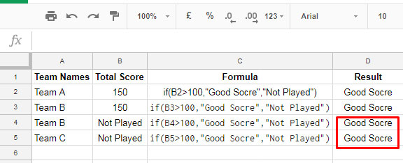
Take a look at Cell D4 and D5. The IF formula checks the value in column B and returns “Good Score” when the score is above 100. However, when the score is below 100 or the team hasn’t played, it should return “Bad Score.” Sadly, the results are incorrect in D4 and D5.

Fortunately, ISNUMBER can solve this issue:

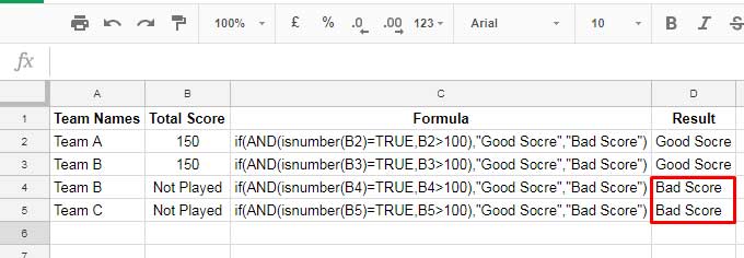
Now, observe the improved results in D4 and D5. You can apply the Google Sheets ISNUMBER function in various scenarios just like these.

That’s all for now. Enjoy exploring the endless possibilities of the ISNUMBER formula in Google Sheets. For more tips and tricks, head over to Crawlan.com. Happy formula-ing, my friends!