How to Master the SUBSTITUTE Function in Google Sheets and Supercharge Your Productivity

Do you want to become a Google Sheets pro? Look no further! In this article, I’ll reveal one of the most powerful and versatile text functions in Google Sheets – the SUBSTITUTE function. Whether you’re a data analyst, a marketer, or a small business owner, mastering this function will revolutionize the way you work with text data. So fasten your seatbelts and get ready to turbocharge your productivity!

Understanding the Magic of the SUBSTITUTE Function

The SUBSTITUTE function in Google Sheets allows you to replace existing text with new text within a string. With this simple yet potent formula, you can effortlessly clean up your text or sentences. Trust me, once you’ve grasped the essence of this function, your life will never be the same again!

Imagine you have a sentence containing the outdated abbreviation “DOB” that you want to replace with “Date of Birth.” Using the SUBSTITUTE function, it’s a breeze. Just follow these steps:

1. Identify the cell that contains the sentence you want to modify. Let’s say it’s in cell A1, and the value is “His DOB is 26-11-2017.”
2. Apply the SUBSTITUTE formula as follows: =SUBSTITUTE(A1,"DOB","Date of Birth").
3. Voilà! The result is “His Date of Birth is 26-11-2017.”

But wait, there’s more! The SUBSTITUTE function offers even greater flexibility. You can also remove specific text from a sentence or apply multiple SUBSTITUTE formulas within a single formula. Let’s explore these possibilities further.

Removing Unwanted Text from a Sentence

Let’s say you have a sentence in cell A1 that reads, “Our Office is Off on coming Saturday, Sunday, and Monday.” But you only want the sentence to mention Saturday and Sunday, without including Monday. No worries! With the SUBSTITUTE function, you can effortlessly remove the unwanted text. Just follow these steps:

1. Identify the cell containing the sentence you want to modify (A1 in this example).
2. Apply the SUBSTITUTE formula: =SUBSTITUTE(A1," , and Monday","").
3. The result? “Our Office is Off on coming Saturday, Sunday.”

Unleashing the Power of Nested SUBSTITUTE Formulas

What if you need to perform multiple substitutions within a single formula? The SUBSTITUTE function has got you covered! By nesting SUBSTITUTE formulas, you can achieve impressive results. Let’s take a look at an example:

1. Imagine you have the following sentence in cell A1: “Our Office is Off on coming Saturday, Sunday, and Monday.”
2. Apply the nested SUBSTITUTE formula: =SUBSTITUTE(SUBSTITUTE(A1," , and Monday","")," ,","b &").
3. The result will be: “Our Office is Off on coming Saturday & Sunday.”

See how easy it is? By combining the power of nested SUBSTITUTE formulas, you can manipulate your text data with unrivaled precision and efficiency.

Removing Special Characters with SUBSTITUTE

The SUBSTITUTE function can also help you remove special characters from your text. For instance, let’s say you have the text “India is My Country” in cell B2, enclosed in double quotes. With the SUBSTITUTE function, you can remove these quotes effortlessly. Here’s how:

1. Apply the SUBSTITUTE formula: =SUBSTITUTE(B2,CHAR(34),"").
2. The result? “India is My Country.”

But what if you want to remove only the first or second occurrence of the double quotes? Not a problem! Just modify the formula slightly:

• To remove the first occurrence: =SUBSTITUTE(B2,CHAR(34),"",1). Result: “India is My Country.”
• To remove the second occurrence: =SUBSTITUTE(B2,CHAR(34),"",2). Result: “India is My Country”.

Supercharge Your Data Analysis with the SUBSTITUTE Function

Now that you’ve learned the ins and outs of the SUBSTITUTE function, it’s time to put it to practical use. As a data analyst, you can leverage the SUBSTITUTE function in combination with other powerful functions to take your data analysis to the next level. Let’s explore an example:

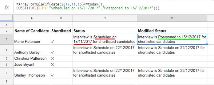
Consider a scenario where you have shortlisted candidates for a final interview. You have a column (D) that indicates the status of the interview. Using the SUBSTITUTE function in combination with other functions, you can automatically update the status based on the scheduled date. Here’s how:

1. Apply the following formula in cell D3: =ArrayFormula(if(date(2017,11,15)<=today(),SUBSTITUTE(C3:C,"Scheduled on 15/11/2017","Postponed to 15/12/2017"))).
2. This formula checks if today’s date is on or after the scheduled interview date (15/11/2017). If it is, it replaces the old date with the new postponed date.
3. The result? The status in column D will be automatically updated based on the current date.

Isn’t that amazing? By combining the SUBSTITUTE function with ARRAYFORMULA and other logical functions, you can streamline and automate your data analysis workflows.

This is just the tip of the iceberg when it comes to the potential of the SUBSTITUTE function. From cleaning up messy data to performing complex text transformations, this function is a game-changer.

So what are you waiting for? Start exploring the possibilities of the SUBSTITUTE function in Google Sheets and unleash your true data ninja potential. For more tips, tricks, and tutorials on mastering Google Sheets, visit Crawlan.com.

Remember, with the SUBSTITUTE function in your arsenal, there’s no text-related challenge you can’t conquer. Happy substituting!