The GESTEP function in Google Sheets is a powerful tool in the Engineering function category. It allows you to determine whether a value (number or date) is greater than a specified threshold value. This function can be used in a variety of scenarios, such as comparing numbers against a threshold or checking if completion dates fall within target dates.
Understanding the GESTEP Function
Let’s dive into the details of the GESTEP function. The syntax is as follows:
GESTEP(value, [step])
value: The value (number or date) to be tested against the threshold.step: The threshold value. By default, it is set to 0.
The GESTEP function returns 1 if the value is greater than or equal to the threshold, and 0 if it is lower.
In some cases, you can achieve similar results using logical operators like the IF function or the comparison operator >= (GTE). However, the GESTEP function provides a more specific approach to handle certain scenarios.
Examples of GESTEP Formulas
To better understand the application of GESTEP, let’s walk through some examples using formulas.
Suppose you have a list of numbers in column A and threshold values in column B. By using the GESTEP function in column C, you can compare each number against its corresponding threshold value. The result and description are provided in adjacent columns.
| A | B | C | D | E | |
|---|---|---|---|---|---|
| 1 | value | step | formula | result | description |
| 2 | 5 | 4 | =GESTEP(A2, B2) | 1 | The step value 4 is less than the value 5. |
| 3 | 10 | 10 | =GESTEP(A3, B3) | 1 | The step value 10 is less than or equal to the value 10. |
| 4 | 5 | 6 | =GESTEP(A4, B4) | 0 | The step value 6 is greater than the value 5. |
| 5 | 10 | =GESTEP(A5) | 1 | If the step value is blank, it is treated as 0. | |
| 6 | -10 | -15 | =GESTEP(A6, B6) | 1 | |
| 7 | 25/05/2020 | 20/05/2020 | =GESTEP(A7, B7) | 1 |
If you have multiple values and step values, you can leverage the ArrayFormula in cell C2 to expand the output. This allows you to check whether numbers or dates in a list are greater than or equal to a single step value.
=ArrayFormula(GESTEP(A2:A7, B2:B7))
Remember to clear the range C3:C7 to allow the array formula to expand the outputs.
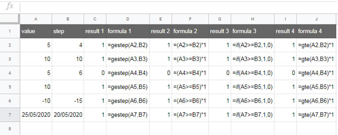
Formula Alternatives – IF Logical and Comparison Operators
Apart from using comparison operators, there aren’t many direct alternatives to the GESTEP function in Google Sheets. The comparison operators offer similar functionalities. You can compare the original formulas in column D with the alternative formulas in columns F, H, and J.
All the formulas mentioned above can also be replaced by array formulas, but we won’t be covering that in this article.
GESTEP Formula within Filter Function in Google Sheets
Let’s conclude this article with an example of combining the GESTEP function with the Filter function in Google Sheets.
Suppose you have a list of tasks in column A, target completion dates in column B, and actual completion dates in column C. You want to filter only the tasks that were completed within the target completion dates.
The following formula combines the Filter and GESTEP functions to achieve this:
=FILTER(A2:A18, GESTEP(B2:B18, C2:C18))
A couple of notes to keep in mind:
- The GESTEP function returns a #VALUE! error if either of the arguments (or both) is a string. Hence, the Filter function automatically skips rows that contain strings in column C.
- The actual completion date in column C should not be left blank; otherwise, it will be treated as 0.
For additional information, in cell B2, the formula used to generate bimonthly dates is as follows:
=FILTER(SEQUENCE(250, 1, DATE(2020, 1, 1), 1), (DAY(SEQUENCE(250, 1, DATE(2020, 1, 1), 1)) = 16) + (DAY(SEQUENCE(250, 1, DATE(2020, 1, 1), 1)) = 1))
That’s all you need to know about using the GESTEP function in Google Sheets. Enjoy exploring the possibilities it offers!
For more Google Sheets tips and tricks, visit Crawlan.com.


