Are you tired of struggling to calculate the return on your bond investment? Well, worry no more! With Google Sheets’ powerful RECEIVED function, you can effortlessly determine the amount received at maturity for fixed-income securities such as bonds. Let me show you how!
To get started, simply open Google Sheets by typing https://sheets.new/ into your browser’s address bar. Once there, you can input the necessary values like settlement date, maturity date, and discount rates to calculate the maturity amount of your bond using the RECEIVED function.
Syntax and Arguments of Google Sheets’ RECEIVED Function
Let’s dive deeper into the technical details and understand the syntax and arguments of the RECEIVED function.
Syntax
RECEIVED(settlement, maturity, investment, discount, [day_count_convention])
Arguments
The RECEIVED function consists of three required arguments and one optional argument:
-
settlement: The settlement date of the security. This is the date when the security is delivered to the buyer after the issue date.
-
maturity: The maturity or expiry date of the security, when it can be redeemed at the face value.
-
investment: The initial investment amount in the security.
-
discount: The discount rate or rate of return of the security.
-
day_count_convention (optional): The day count basis used for calculation. The default value is 0.
For a complete understanding of the day count conventions, refer to the table below:
| day_count_convention | Description |
|---|---|
| 0 | US (NASD) 30/360 |
| 1 | Actual/Actual |
| 2 | Actual/360 |
| 3 | Actual/365 |
| 4 | European 30/360 |
An Example of Using the RECEIVED Function in Google Sheets
Let’s take a practical example to illustrate how the RECEIVED function works in Google Sheets.
Suppose you have a bond with an initial investment of $10,000 and a discount rate of 4.5%. The settlement date is 1-Apr-2014, and the maturity date is 01-Jan-2020.
To calculate the maturity amount, use the following formula:
=RECEIVED(date(2014, 4, 1), date(2020, 1, 1), 10000, 4.5%)Here’s a visual representation of the example:
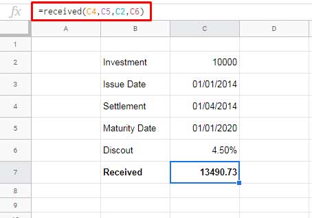
Please note that in this example, we have omitted the day_count_convention, so it is considered as 0, which corresponds to the US (NASD) 30/360 convention.
Possible Errors in Using the RECEIVED Function
While using the RECEIVED function in Google Sheets, you may encounter two possible errors: #VALUE! and #NUM!. Let’s see why these errors occur:
Reasons for the #VALUE! Error:
- Invalid settlement or maturity date formats.
- Investment amount and discount percentage formatted as texts.
Reasons for the #NUM! Error:
- Missing investment amount or discount percentage in the formula.
- Investment or discount amount being less than or equal to zero.
- Invalid day_count_convention base. It should be omitted or one of the numbers 0, 1, 2, 3, or 4.
- Settlement date being greater than or equal to the maturity date.
That’s it! Now you have the power to effortlessly calculate bond maturity using Google Sheets. Enjoy the simplicity and accuracy of the RECEIVED function and make your financial analysis a breeze!
For more exciting tips and tricks on Google Sheets, visit Crawlan.com. Happy calculating!


