I’ve got a secret to share with you, and it’s about a little-known gem called the To_text function in Google Sheets. Trust me, once you discover its power, you’ll wonder how you ever lived without it. Let me take you on a journey of its usefulness and show you how it can solve some of your most frustrating data import and manipulation problems.
Unleashing the Magic of the To_text Function
In Google Sheets, you may already know about using an apostrophe (‘) to convert numbers, dates, or any value to text without losing its format. Well, the To_text function does just that, but in a more efficient and elegant way.
Here’s the syntax of the Google Sheets To_text function:
TO_TEXT(value)
For example, let’s say you have a column with a mix of dates, text strings, currency values, and blank rows. You want to import only the rows that contain values. That’s where the To_text function comes to the rescue.
Imagine the scenario: You have a column with various cell formats, and you only wish to import the meaningful rows. By using the To_text function in combination with Query and Importrange, you can achieve just that.
Let’s start with some basic tips on how to use the To_text function in Google Sheets.
Harnessing the Power of the To_text Function
With the To_text function in your arsenal, you can convert date, currency, time, and number formats to text while still retaining their original formatting. It’s as simple as using the To_text formula.
Take a look at the following example where the To_text formulas convert various formats to text while preserving their original layouts:

But wait, there’s even more to it! You can use the To_text function in an Array Formula as well. Instead of using multiple formulas, the To_text function supports arrays effortlessly. For instance, try the formula below:
=ArrayFormula(to_text(A13:A17))
Utilizing the To_text Function in Query
Now that you’re getting the hang of it, let’s dive into the power of the To_text function within Query. This functionality can prove to be immensely useful when consolidating rows or importing specific data.
While the use of Regex in the Query Match clause is a great way to filter specific values in a column, not everyone is an expert in Regex. Thankfully, the To_text function in Query can make things much simpler.
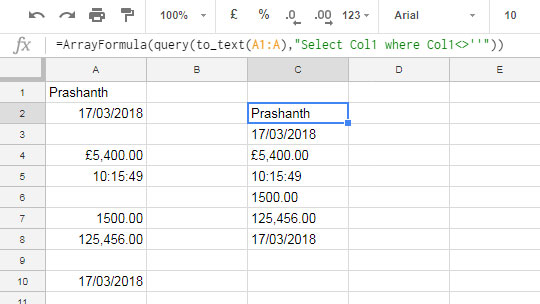
Imagine having a column with mixed data types and wanting to filter only the rows that contain values. When using Query in this scenario, things can become quite puzzling. So, what’s the solution?
By first converting the values in the column to text using the To_text function, you can then use the <>'' operator in the Where clause to filter only the rows that are not equal to empty space.
Remember to use the Array Formula when applying the To_text function in an array.
Here’s an example of how you can use the To_text function in Query:
Leveraging the To_text Function in Importrange
The To_text function in Importrange can also work wonders. Simply refer to the formula mentioned earlier, but make sure to change the range within the Importrange formula to suit your needs. It’s as easy as that!
For example:
=ArrayFormula(query(to_text(IMPORTRANGE("Blah.. Blah..Blah..","Sheet1!A1:A")),"Select Col1 where Col1<>'"))
In Conclusion
As you can see, Google Sheets is equipped with a myriad of powerful functions, and the To_text function certainly has its place among them. By understanding its capabilities, you can overcome data import obstacles and streamline your workflows.
So, why not give it a try? Embrace the To_text function in Google Sheets and unlock its potential to make your data manipulation tasks a breeze. Trust me, you won’t regret it!
P.S: If you’d like to explore more Google Sheets tips and tricks, head over to Crawlan.com for a treasure trove of knowledge. Happy exploring!


