Are you tired of searching for ways to insert check boxes and tick marks in your Google Sheets? Look no further! In this article, we will explore the best methods to insert these symbols and make your Sheets more interactive.
The Traditional Approach: Using the CHAR Function
Many Google Sheets users effectively use the CHAR function to insert check boxes and tick marks. You can follow this method too, as there is no other option available at this time. Here is the best way to insert these symbols in Google Sheets.
Update: There is a new method now available in Google Sheets to insert check boxes without using the CHAR function. It’s using data validation or through the Insert menu. I’ve detailed this at the end of this tutorial under the title “Tick Box Using Data Validation Alone.”
You can use the CHAR function alone or in combination with Data Validation to insert check boxes and tick marks in Google Sheets. Data Validation is only required if you want a user to make a choice.
Don’t worry; we will guide you through all these aspects and additionally teach you how to use check boxes and tick marks in Google Sheets calculations.
How to Insert Check Box and Tick Mark Symbols in Google Sheets
First, let’s take a look at how to insert check boxes in Google Sheets. You can use the below formulas as per your requirement:
A) Formula 1: =char(9745)
B) Formula 2: =CHAR(9744)
C) Formula 3: =char(9746)
Now if you want just tick mark and check mark symbols, you can use the following formulas:
A) Formula 1: =char(10006)
B) Formula 2: =char(10004)
No need to always use these formulas. You can apply all the above formulas in one sheet and afterward, you can directly copy the symbols from here and paste them in any cell, any sheet, and even any Google Sheet file.
But why is data validation required to insert check marks and check boxes in Google Sheets?
If you want users to make tick marks and check boxes similar to Excel, the best workaround in Google Sheets is to use a drop-down menu using the data validation feature.
Using Data Validation to Insert Check Boxes and Tick Marks in Google Sheets
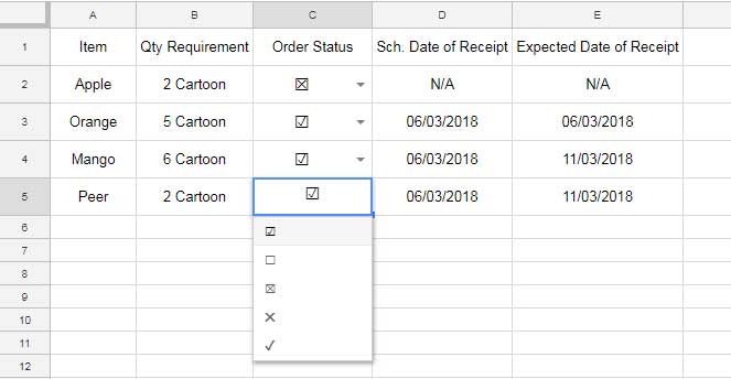
In Sheet 1, apply all the above formulas one by one in the range A1:A5.
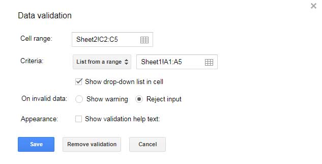
In Sheet 2, I am applying the following data validation rule in the range C2:C5. You can use any column in your sheet. This is just an example.
To apply data validation, select the cell range C2:C5 and go to the menu Data > Data validation. Set the data validation rule as follows:
This way, you can insert check boxes and tick marks in Google Sheets. Now, let’s move on to using these symbols in calculations.
Filtering Data Based on Tick Mark / Check Mark Symbols in One Column in Google Sheets
Let’s say you have a dataset and want to filter the data based on column C check boxes. You can use the following filter formula:
=filter(A2:E5,C2:C5=CHAR(9746))
You can also use this formula by copy and pasting the check box in the formula as criteria:
=filter(A2:E5,C2:C5="☒")
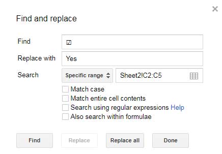
Replacing Tick Marks with “Yes” or “No” in Google Sheets
To replace all tick marks and check boxes with any value, you can use Google Sheets’ find and replace command (Ctrl+F). For example, you can replace the tick box with “Yes”. Just copy and paste the check box inside the field against “Find”.
Tick Box Using Data Validation Alone in Google Sheets (The Quickest Way of Inserting Tick Boxes)
This is a very simple approach and looks awesome. This is new in Google Sheets and hidden inside the Data Validation. Let’s see how to insert this new kind of Tick Boxes in Google Sheets.
Steps:
- Select the cells where you want the tick boxes to appear.
- Go to the menu Data > Data validation and select Tick Box and click Save. That’s it.
The tick box will be inserted in the selected cells. See the example below where I’ve inserted tick boxes in the cell range A1:A8. Then I’ve selected two tick boxes by just clicking on them.
This is the fastest way to insert check boxes and tick marks in Google Sheets.
When you click a tick box to mark it, the cell value becomes Boolean TRUE. Otherwise, it’s FALSE. In the above example, the values in Cell A2 and A5 are TRUE. So in Filter, Query, and also in Logical Test, you can use TRUE or FALSE as a condition.
Tick Box Based Example Formulas on the Above Flower Data
Here are some example formulas to use with the new data validation Tick Box:
How to use the new data validation Tick Box in a Logical IF statement?
=if(A2=TRUE,B2,"NOT SELECTED")
How to use the Tick Box in FILTER?
=FILTER(B1:B8,A1:A8=FALSE)
How to use the Tick Box in Google Sheets Query?
=query(A1:B8,"Select B where A<>TRUE")
That’s all about check boxes, tick boxes, tick marks, and tick symbols in Google Sheets. If you have any other questions, stay tuned for more tutorials from Crawlan.com. Enjoy!


