How to Link a Specific Sheet in Google Sheets

Learning how to link a specific sheet in Google Sheets is a useful skill that allows you to share specific sheets with others without compromising the entire Google Sheets file.

The beauty of using Google Sheets lies in its ability to share or collaborate with multiple people. It’s convenient and responsible as it allows you to track all the changes made to the sheet.

Google Sheets is used worldwide by people of all ages, from students to working adults. It’s essential to navigate and master the features of Google Sheets. Sometimes, you may have multiple sheets or tabs in Google Sheets and want to link a specific sheet for reference.

Here are some tips to easily link a specific sheet in Google Sheets!

Copy and Paste the Link of the Specific Sheet

The easiest way is to copy and paste the specific link of the Google Sheet or tab. You can either copy the URL from the top of your browser window or use the share button.

Example 1

For instance, you’re planning to attract more capital for your business. Potential investors have requested information about the company to better understand your organization.

However, all the information is scattered across different tabs, or even different Google Sheets files.

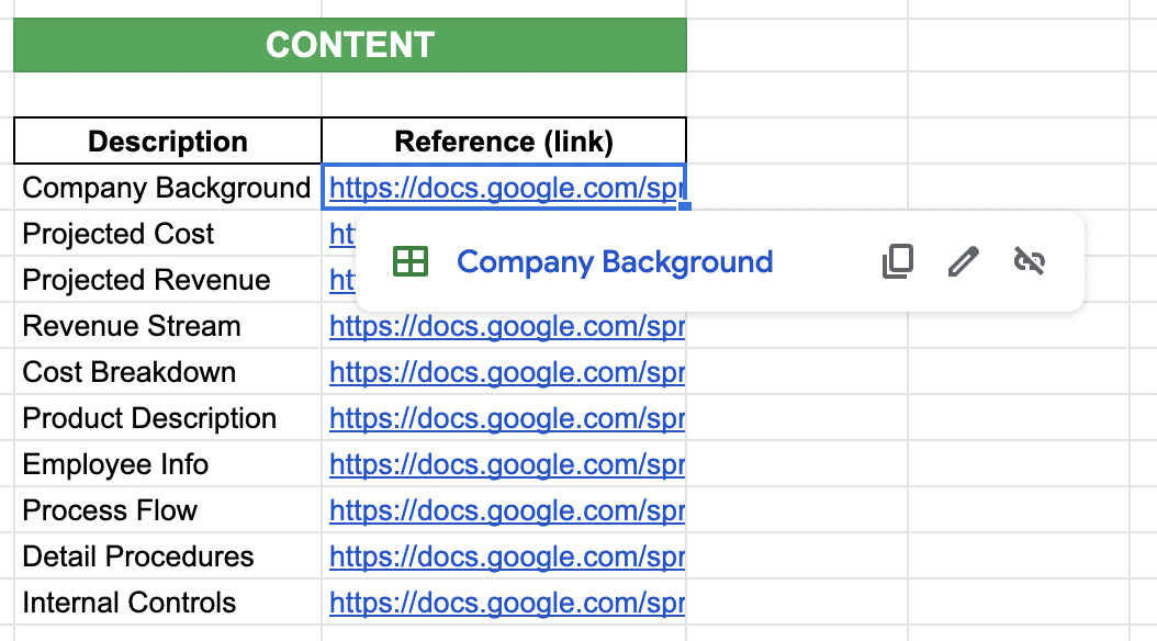
By linking a specific sheet in Google Sheets, we can create a table of contents to link all the main information in a single tab for clarity. This way, potential investors can see different aspects of your company in an organized manner.

1. The simplest way is to copy the URL from the top of your browser window.
2. What’s great is that the URL is specific to that tab in Google Sheets.
3. Another way to copy the specific link would be via the “Share” button.
4. You can copy the link from the “Get Link” section by clicking “Copy.”
5. Using this method, you can limit the person with the link to only view the Google Sheets file or tab.
6. Once the content tab is completed, all the important sheets or tabs are linked. Now, potential investors can easily access specific sheets from a single tab.

Example 2

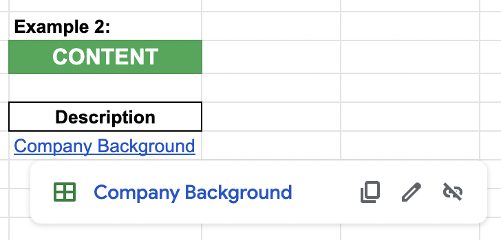
Some of you may think that the sheet looks cluttered with many links in the preview. Here’s a fancier way to link specific sheets in Google Sheets.

1. First, right-click on the desired cell and click on “Insert link.”
2. A pop-up box will appear. Insert the word you want to display in the cell and paste the specific sheet link.

Once you have clicked “Apply,” it will appear like this:

This way, the spreadsheet looks cleaner and more professional, without exposed links.

Import Data from a Specific Sheet into a New Google Sheets

Imagine you have a business idea and are planning to get a loan from the bank. The banker has requested a detailed business plan to review. A business plan will help them decide if the business idea is viable and capable of repaying the loan.

Your business information is usually scattered across different tabs and Google Sheets files. Moreover, you want to compile all the information into a single business plan using Google Sheets.

Instead of simply inserting a link or linking the cell to a specific sheet, we can import data from the specific sheet into a new Google Sheets.

We will use the IMPORTRANGE function for this. This function copies data from one spreadsheet to another. You might be wondering what’s the difference compared to manually copying the data into a new Google Sheets, right?

The beauty of using the IMPORTRANGE function is that it copies all the changes made in the original sheet. So, there’s no need to constantly copy the data into the sheet every time there are updates.

If you’re not familiar with the IMPORTRANGE function, feel free to check out the anatomy of the function and other examples of its usage!

Example 1

1. First, select the cell where you want to enter the function. In this case, it’s C13.
2. Start your function with an equal sign (=), followed by the function name, IMPORTRANGE, then an opening parenthesis (.
3. Now, we will open and close quotation marks, inside of which will be the link to the specific sheet.
4. Right after the quotation mark, add a comma, followed by another quotation mark.
5. Add the range field you want to copy. It should look like this, ‘Projected Revenue’!A1:H10. This means we will import data from a sheet named “Projected Revenue” covering cells A1 to H10.
6. Add another quotation mark, followed by a closing parenthesis) and press Enter.
7. Your sheet will look like this:

Note that only the cells are imported with the data. Font size, borders, and other elements won’t be copied or can’t be copied. Additionally, the imported data will use the default settings of the new spreadsheet.

Therefore, we can enhance the data by making the headers bold or adding lines to the cells.

How to Protect and Hide Specific Sheets

As you already know, by sharing links to specific sheets or using the IMPORTRANGE function, the URL of our original sheet is exposed.

This means that other important data from the specified sheet would also be shared or viewed by others. Furthermore, viewers can also edit the original Google Sheets if the tabs or cells are not protected using the sheet protection tool.

It’s essential to learn how to protect our Google Sheets and data using these three methods.

And there you have it! Two different ways to link a specific sheet in Google Sheets to make your life easier!

Don’t forget to check out other interesting functions in Google Sheets to enhance and simplify your daily work!

To learn more about Google Sheets and other marketing tips, you can visit Crawlan.com.