Have you ever found yourself needing to reference data from one sheet to another, or even from one spreadsheet to another, in order to create a combined master view? This allows you to consolidate information from multiple spreadsheets into a single one.
Another common scenario may require a backup spreadsheet that copies the values and format from the source file, but not the formulas. Some users may also want their master document to update automatically, according to a predefined schedule.
If you’re struggling to find the solution to these tasks, you’ve come to the right place. In this article, I’ll share some tips on linking data from other sheets and spreadsheets, as well as alternatives to do so. Finally, I’ll provide a comprehensive comparison of the mentioned approaches so that you can evaluate and choose them with confidence.
How to Reference Data from Other Sheets or Tabs – What are the Options?
There are several cases and ways to reference data in Google Sheets. You can reference another spreadsheet in Google Sheets, a cell or range of cells, as well as columns and rows. Additionally, you may need to import data from one spreadsheet/sheet to another based on certain criteria, or even combine data from multiple sheets into a single view.
Google Sheets offers a few native options to reference data, including the IMPORTRANGE function. However, you should keep in mind that:
- Google Sheets’ native functions and options only allow you to reference data, not import it.
Yes, Google Sheets does not provide a feature to actually import data from one spreadsheet/sheet to another, even though the name of the IMPORTRANGE function suggests otherwise. They only reference a specified range, meaning that if your source sheet data is not available, you won’t have access to it in your destination sheet. This is a drawback. So, if you need to import data (cell range, columns, or rows) from one sheet to another, you’ll have to opt for a third-party solution, either a web app or a Google Sheets add-on. Or you can simply copy the data from another spreadsheet into Google Sheets, but that’s more for beginners :)
Below, we’ll cover both the native options in Google Sheets for referencing data and third-party tools for importing data between Google Sheets. Let’s start with the former.
If Excel spreadsheets are your priority, check out our blog article on how to link sheets in Excel.
You can use formulas to reference columns or rows to link cell ranges between different sheets of the same spreadsheet. We’ll discuss this later in this section. Let’s first start with more advanced cases for linking sheets using the FILTER function in Google Sheets.
Linking Google Sheets Tabs Based on Criteria
Let’s say you want to filter your data set based on specific criteria and import the filtered values into another sheet. You can do this using the FILTER function, which was introduced in the above example. Here’s the syntax:
=FILTER(data_set,criterium1, criterium2,...)
data_set– a range of cells to filter.criterium– the criteria for filtering the data set.
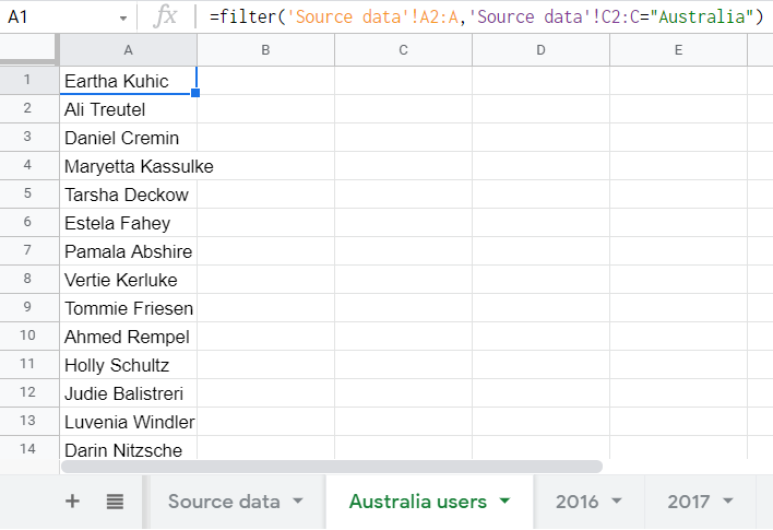
For example, let’s filter users by country, Australia, and import the results into another sheet.
Here’s what our formula will look like:
=filter('Source data'!A2:A,'Source data'!C2:C="Australia")
Read the Google Sheets FILTER function to discover more filtering options.
How to Import Data from Multiple Sheets into a Single Column
Let’s look at an example where you need to link data from multiple columns of different sheets into one.
In my example, I have three different tabs with sales data: Sales 1, Sales 2, and Sales 3. My task is to gather all customer names into the sheet called “All Customers.”
For this, I’ll use this formula:
={
  "All Customers";
  FILTER('Sales 2'!C2:C, LEN('Sales 2'!C2:C) > 0);
  FILTER('Sales 1'!C2:C, LEN('Sales 1'!C2:C) > 0);
  FILTER('Sales 3'!C2:C, LEN('Sales 3'!C2:C) > 0)
}
Where:
- “All Customers” is the name given to my column,
FILTER('Sales 1'!C2:C, LEN('Sales 1'!C2:C) > 0)means that I’m taking all data from column C of “Sales 1”, excluding values equal to or less than 0.
Result: I get the names of all my customers from three different sheets gathered into a single column.
One advantage of this approach is that I can change the names of my data source sheets (from where I retrieve the data), and they will be automatically updated in the formula!
Let’s see how it works:
At the same time, there is a better option to consolidate your data from multiple Google Sheets spreadsheets into a single master view – we’ve covered it in this section.
The options presented above work for referencing data between sheets of a single Google Sheets document. If you need to link to another spreadsheet (sheet or tab of another Google Sheets document), then you need IMPORTRANGE. It is a function in Google Sheets that allows you to import a range of data from one spreadsheet to another. However, it doesn’t actually import the data, only references it.
To reference another sheet in a Google Sheets spreadsheet, follow these instructions:
- Go to the spreadsheet from which you want to export data. Copy its URL.
- Open the sheet to which you want to download the data.
- Place your cursor in the cell where you want your imported data to appear.
- Use the following syntax:
=IMPORTRANGE("spreadsheet_url", "cell_range")
spreadsheet_urlis the Google Sheets link to another sheet, which you copied previously to fetch the information.cell_rangeis an argument you enclose in quotation marks to specify the sheet and range from which you want to download the data.
For example:
- Use “new students!B2:C” to name the sheet and range from which to get information.
- Use “A1:C10” to specify only a range of cells. In this case, if you don’t specify the sheet from which to import, the default behavior is to download the data from the first sheet of your spreadsheet.
You can also use:
=IMPORTRANGE(B19, "B2:C6")
If B19, in this case, contains the URL of the necessary spreadsheet to link the data.
Note: Using IMPORTRANGE assumes that your destination spreadsheet needs permission to retrieve data from another (the source) document. Every time you want to import information from a new source, you’ll have to authorize this action. After granting access, anyone with edit rights in your destination spreadsheet will be able to use IMPORTRANGE to import data from the source. The access will be valid as long as the person who provided it is present in the data source. To learn more about this Google Sheets function, check out our IMPORTRANGE tutorial.
In my case, my formula looks like this:
=IMPORTRANGE("spreadsheet_url","new students!B2:C")
Or:
=IMPORTRANGE("spreadsheet_url","B2:C")
because “new students” is the only sheet I have in my spreadsheet.
However, the IMPORTRANGE solution has several drawbacks. One that I’ll mention concerns a negative impact on overall spreadsheet performance. You can search for IMPORTRANGE in the Google Community Forum to see a number of threads explaining the issue in more detail. Basically, the more IMPORTRANGE formulas you have in your spreadsheet, the slower the overall productivity will be. The spreadsheet will stop working or take a long time to process and display your data.
How to Link Two Google Sheets Without the IMPORTRANGE Function
Although using IMPORTRANGE is one of the most common methods to link two different sheets in Google Sheets, there are also other options:
- Google Sheets API. This is an advanced method that may not be suitable for most users as it requires programming skills to connect one spreadsheet to another. However, it’s also possible to use this method. Fortunately, the other two methods in our list are suitable for non-technical people as well.
- Data Integration Solutions. These are specialized tools that can automatically connect various applications and automate data flows. They can also be used to link two Google Sheets sheets. One of them is Coupler.io, which is also available as an add-on. I recommend trying it out as it is very user-friendly. I’ll explain how to link two different Google Sheets sheets with Coupler.io in the next section.
- Third-Party Add-ons. There are different add-ons available on the Google Workspace Marketplace that can help you extend native functionalities. For example, Coupler.io and Sheetgo allow you to link two Google Sheets sheets without any formulas. That’s why they are even called an “IMPORTRANGE alternative.”
As mentioned from the beginning, there is no native way to import data from one sheet or spreadsheet to another in Google Sheets. So, to get this job done, you’ll need a Google Sheets add-on or an ETL (Extract, Transform, Load) tool. Coupler.io offers both options as a whole!
Coupler.io is a report automation platform to convert raw data into simple reports. The platform offers multiple integrations to automate data import. It supports 50+ sources and 6 destinations, including Google Sheets.
With Coupler.io’s Google Sheets integration, you can link sheets and spreadsheets – let’s see how it works.
How to Import Data from Another Google Sheet or Spreadsheet
Click “Continue” in the form below, where we’ve already selected Google Sheets as the source and destination.
You can sign up for free with your Google account. Then, go through the following steps to set up the integration.
Step 1. Extract Data from a Source Sheet
- Log in to your Google account.
- In your Google Drive, select a spreadsheet and a sheet from which to import data. You can select multiple sheets if you want to merge data into a master view.
Next, optionally specify a range to export the data, for example, A1:Z9, if you don’t need to extract data from an entire sheet.
Coupler.io allows you to load data from multiple sheets of a single spreadsheet. If you want to combine data from multiple spreadsheets, you can click “Add Another Source” and connect another spreadsheet to import data.
Step 2. Transform Data
In the next step, you can preview and even transform the data to be imported. Coupler.io allows you to:
- Hide/show columns, change column names, and types.
- Filter and sort data.
- Create new columns using supported formulas.
Step 3. Manage Data to Load into a Destination Sheet
- Log in to your Google account.
- Select a file on your Google Drive and a sheet to load the data into. You can create a new sheet by entering a new name.
You can also modify the first cell to import your range of data (cell A1 is set by default) and change the data import mode: “replace” your previous information or “append” new rows below the last imported entries. You can also enable the “Last Updated Column” feature if you want to add a column to the spreadsheet with information about the last date and time of the update.
Once you’re done with this step, you can run the import immediately and link your Google Sheets spreadsheet to another sheet. If you want to automate data import on a schedule, check the instructions in the next section.
How to Sync Two Google Sheets According to a Schedule Without Formulas
Coupler.io allows you to easily sync two Google Sheets according to a custom schedule. Once you’ve completed the steps described above and your Coupler.io importer is almost ready, you can specify your preferences for updating the data.
Enable “Automatic Data Update” and customize the schedule.
- Select the interval (every 15 minutes to every month).
- Select the days of the week.
- Select time preferences.
- Schedule the time zone.
Finally, click “Save and Run” to sync two Google Sheets. The latest information from the data source will be automatically transferred to the destination sheet during the next scheduled update.
Note: You can also use Coupler.io as a Google Sheets add-on for quicker access to the tool within your spreadsheet. To do that, install it from the Google Workspace Marketplace and set it up as we described above. Watch our YouTube video on installing the Coupler.io add-on and setting up a Google Sheets importer.
How to Reference a Cell in Another Workbook in Google Sheets with Coupler.io
Coupler.io allows you not only to reference another workbook in Google Sheets but also to import an exact range of cells that corresponds only to the specified range. For example, you want to extract data from range A1:C8 from one workbook and insert it into range C1:E8 in another workbook. For this, perform the configuration described above, but also specify the following parameters:
Source Sheet Range(Step 1) – here, you’ll need to specify the range of cells from which to import data. In our example, A1:C8.Destination Cell/Range Address(Step 3) – here, you’ll need to specify the range of cells where to import the data. In our example, C1:E8.
Click “Save and Run” and welcome your data into the specified range of cells.
Note: If you want to import data between sheets, the source and destination spreadsheet ID will be the same.
Which Option Works Best in Google Sheets for Links to Another Sheet or Tab?
Below, I’ve prepared a comparative table that briefly explains the advantages and disadvantages of using native functionalities versus Coupler.io when linking data between spreadsheets.
| Google Sheets Native Features | Coupler.io | |
|---|---|---|
| Google Sheets Link Type | Decent | Excellent |
| Large Data Volumes | OK | Very good |
| Update Frequency | Acceptable | Excellent |
| Calculation Processing Time | Acceptable | Excellent |
| Performance in Formulas-Heavy Spreadsheets | Acceptable | Excellent |
| Permission/Access Handling | – | Excellent |
| Data Backup | – | Excellent |
If you’re interested in comparing IMPORTRANGE and Coupler.io in terms of linking sheets in a spreadsheet, check out our dedicated blog article on IMPORTRANGE in Google Sheets.
It’s also worth noting that you can use Coupler.io to import Excel files as well as Excel and Google Sheets files.
Can I Import Data into Google Sheets from Another Sheet While Keeping the Formatting?
Unfortunately, none of the options above allow you to import cell or cells’ formatting when you reference another Google Sheets workbook. The logic of Google Sheets’ native options (IMPORTRANGE, FILTER, and others) does not provide for the actual transfer of formatting. They only reference and display the data from the source cells. Coupler.io is the only option that copies the data from the source, but it imports only raw data without any formatting. However, you can still use the benefits of Google Apps Script to create a custom function for your needs. For example, the following script allows you to transfer data from one sheet or spreadsheet to another:
function importTable() {
  // Source spreadsheet
  var srcSpreadSheet = SpreadsheetApp.openById("insert_source_spreadsheet_id");
  var scrSheet = srcSpreadSheet.setActiveSheet(srcSpreadSheet.getSheetByName("insert_source_sheet_name"));

  // Destination spreadsheet
  var destSpreadSheet = SpreadsheetApp.openById("insert_destination_spreadsheet_id");
  var destSheet = destSpreadSheet.setActiveSheet(destSpreadSheet.getSheetByName("insert_destination_sheet_name"));

  destSheet.clear();

  // Extract data and formatting from the source sheet
  var range = scrSheet.getRange(1, 1, 48, 32);
  var values = range.getValues();
  var background = range.getBackgrounds();
  var banding = range.getBandings();
  var mergedRanges = range.getMergedRanges();
  var fontColor = range.getFontColors();
  var fontFamily = range.getFontFamilies();
  var fontLine = range.getFontLines();
  var fontSize = range.getFontSizes();
  var fontStyle = range.getFontStyles();
  var fontWeight = range.getFontWeights();
  var horAlign = range.getHorizontalAlignments();
  var textStyle = range.getTextStyles();
  var vertAlign = range.getVerticalAlignments();

  // Put data and formatting into the destination sheet
  var destRange = destSheet.getRange(1, 1, 48, 32);
  destRange.setValues(values);
  destRange.setBackgrounds(background);
  destRange.setFontColors(fontColor);
  destRange.setFontFamilies(fontFamily);
  destRange.setFontLines(fontLine);
  destRange.setFontSizes(fontSize);
  destRange.setFontStyles(fontStyle);
  destRange.setFontWeights(fontWeight);
  destRange.setHorizontalAlignments(horAlign);
  destRange.setTextStyles(textStyle);
  destRange.setVerticalAlignments(vertAlign);

  // Repeat to put merged ranges in place
  for (var i = 0; i < mergedRanges.length; i++) {
    destSheet.getRange(mergedRanges[i].getA1Notation()).merge();
  }

  // Repeat to get column width from the source to destination
  for (var i = 1; i < 18; i++) {
    var width = scrSheet.getColumnWidth(i);
    destSheet.setColumnWidth(i, width);
  }

  // Repeat to get row height from the source to destination
  for (var i = 1; i < 27; i++) {
    var height = scrSheet.getRowHeight(i);
    destSheet.setRowHeight(i, height);
  }
}
You need to go to “Extensions > Apps Script.” Then, insert the script into the Code.gs file and specify the required parameters:
- Source and destination spreadsheet IDs
- Source and destination sheet names
(If you’re importing data between sheets, the source and destination spreadsheet ID will be the same)
When you’re ready, click “Run,” and your data, including formatting, will be imported into the destination sheet.
Note: This solution may not fit your project, so you’ll need to update the script according to your needs.
Whichever option you choose, make sure to consider all the advantages and disadvantages of both and choose the right one to achieve the best result.
If you only have a few records in your spreadsheet and few formulas, you can go for a formula-based approach, including IMPORTRANGE provided by Google Sheets. This will work for regular reporting or lower-level analytics.
However, if you have lots of data and there are several calculations in your document, you should go for the data import method instead of referencing it. Coupler.io will be a more stable solution in this case. It will ensure a seamless data transfer and guarantee that you have access to the data even if the data source is damaged or unavailable. Choose wisely and good luck!


