Have you ever encountered the need to highlight specific cells in your Google Sheets based on certain conditions? Conditional formatting can be a powerful tool for this task. However, when the cells to highlight and the conditions are in different sheets, things can get a bit more complicated. But fear not! In this article, we will delve into the world of relative references in conditional formatting and learn how to apply them in Google Sheets.
Relative Cell Reference in Conditional Formatting in the Same Sheet
Let’s start with the basics. The relative cell reference allows us to use a single conditional format formula to apply to an entire row or column range. This eliminates the need to create separate formula rules for each cell or row/column.
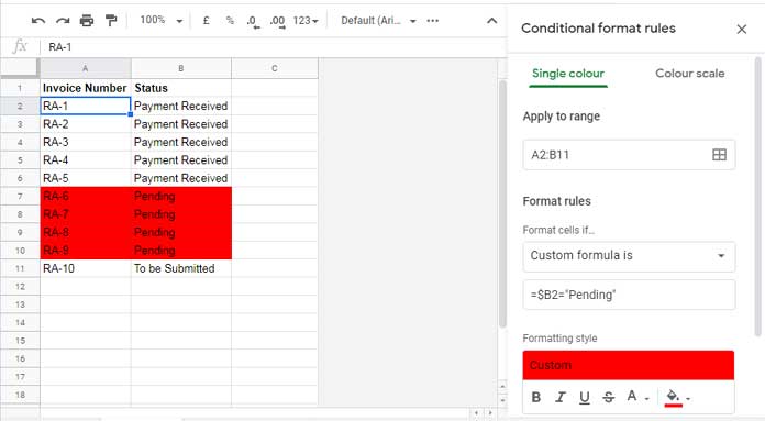
For example, let’s say we want to highlight values in column A if the corresponding values in column B are marked as “Pending.” Here’s the custom formula you would use in the conditional formatting menu:
= B2="Pending"The trick here is to take note of the “Apply to range” field within the “Conditional format rule” panel. By entering A2:A, the formula for the first cell in the range will automatically be applied to the selected range.
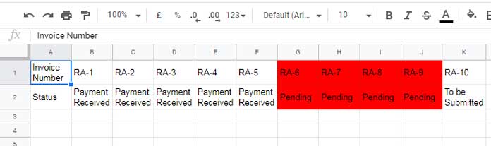
What if you want to highlight both columns A and B? Simply change the “Apply to range” to A2:B. However, to ensure the formula works as intended, make the column (letter) absolute and the row (number) relative in the formula:
= $B2="Pending"And just like that, you can easily highlight values based on specific conditions within the same sheet.
Relative Cell Reference in Conditional Formatting in Two Sheet Tabs
But what if the cells you want to highlight are in one sheet, while the conditions you want to apply are in another sheet? This is where things get a little tricky. However, we have a workaround: the Indirect function.
To illustrate this, let’s consider a scenario where the invoice numbers are in column A of “Sheet1,” and the corresponding statuses are in column B of “Sheet2.” In this case, the cell range to highlight is in one sheet, while the conditions are in another sheet. The formula you might initially think to use, such as Sheet2!B2="Pending", won’t work as conditional formatting rules in Google Sheets are only applicable within the same sheet.
To overcome this limitation, we can use the Indirect function. This function allows us to refer to cells in another sheet within the conditional formatting formula. Here’s an example of how to use it:
= indirect("'Sheet2'!"&address(row(B2),column(B2),4))="Pending"With this formula, you can apply relative cell reference highlighting to an entire row or column in “Sheet1” based on conditions in “Sheet2.”
To highlight multiple rows in “Sheet1” based on the same conditions in “Sheet2,” you can modify the formula as follows:
= indirect("'Sheet2'!"&address(row(B$2),column(B$2),4))="Pending"And there you have it! The Indirect function enables you to apply conditional formatting across different sheets within the same file.
To visualize these concepts further, check out the images here and here.
Now you’re equipped with the knowledge of how to use relative references in conditional formatting in Google Sheets. This can greatly enhance your ability to highlight specific cells based on certain conditions, even when those cells are in different sheets. Happy formatting!
Additional Resources


