With the help of an array formula (helper column) in the source data, you can easily sum Min or Max Values in Pivot Table in Google Sheets. In this article, we’ll address the issue you may face when using the functions MIN or MAX within the pivot table editor.
The Grand Total Issue
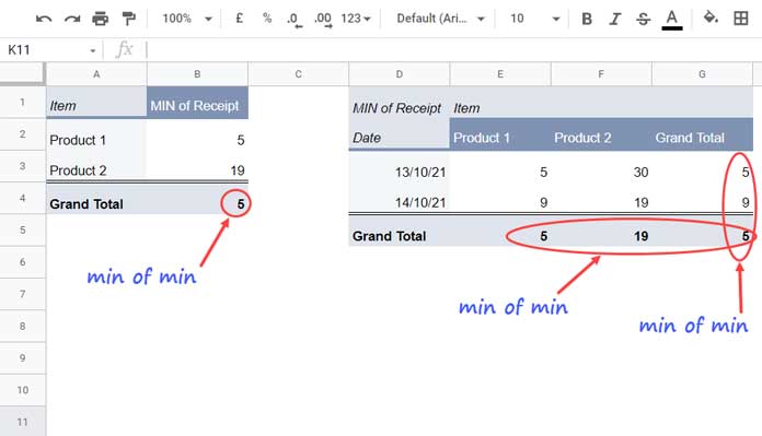
When you enable “Show Totals” of COLUMNS or ROWS in the Pivot Table editor and use either of the functions, Min or Max, in the VALUES field, you may encounter a problem. The Grand Total columns may return Min of Min or Max of Max. This is not what you want. You want the Sum of Min or Sum of Max in Grand Totals.
What we want:
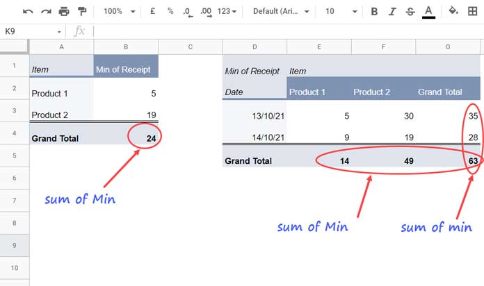
What we usually get:
Please take a moment to understand the difference between the pivot tables in the above images. Now let’s explore the solution.
How to Sum Min Values in Pivot Table in Google Sheets?
We will prepare two pivot tables to demonstrate the solution. In the first example, we will group the data by Item, and in the second example, we will group the data by Date and Item.
Example 1 (Pivot Table 1)
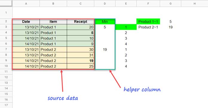
In this example, we have the following data:
To achieve the desired result, follow these settings in the Pivot Table Editor:
- Data Range: A2:D10
- Rows: Item – Show Totals
- Columns: None
- Values: Min – Use the helper column range D2:D10
Here are the formulas to generate the helper Min column:
In cell E3, insert the following running count array formula:
=ArrayFormula(countifs(row(B3:B10),"<="&row(B3:B10),B3:B10,B3:B10))
In cell F2, use the below Query to group the field Item and return the minimum receipt of the item in each group:
=ArrayFormula(query({B2:B10&"~"&1,C2:C10},"Select Col1,min(Col2) group by Col1 label Col1'',min(Col2)''",1))
Now you can combine these formulas and use them in cell D2 as follows:
={"Min";ArrayFormula(IFNA(vlookup(B3:B10&"~"&countifs(row(B3:B10),"<="&row(B3:B10),B3:B10,B3:B10),query({B2:B10&"~"&1,C2:C10},"Select Col1,min(Col2) group by Col1 label Col1'',min(Col2)''",1),2,0)))}
Please note that you can modify the field labels in the pivot report to suit your needs.
Example 2 (Pivot Table 2)
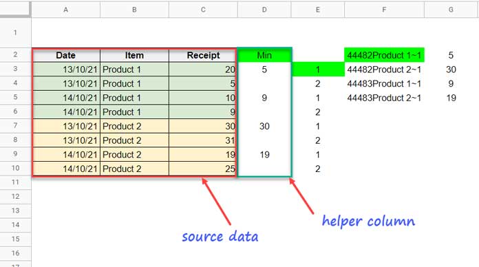
In this example, we will group the data by Date and Item. The data and pivot table will look like this:
To achieve the desired result, make the following changes:
Changes in the Formulas
Running Count in E3:
=ArrayFormula(countifs(row(B3:B10),"<="&row(B3:B10),A3:A10&B3:B10,A3:A10&B3:B10))
Query in F2:
=ArrayFormula(query({A2:A10&B2:B10&"~"&1,C2:C10},"Select Col1,min(Col2) group by Col1 label Col1'',min(Col2)''",1))
Vlookup in D2:
={"Min";ArrayFormula(IFNA(vlookup(A3:A10&B3:B10&"~"&E3:E10,F2:G5,2,0)))}
Changes within the Pivot Table Editor
Rows: Date – Show Totals
Columns: Item – Show Totals
Values: Min – Use the helper column range D2:D10
Summarize by: Sum
How to Sum Max Values in Pivot Table in Google Sheets?
To sum max values in a Pivot Table in Google Sheets, follow the same steps as above, but replace the MIN function with MAX in the Query. Additionally, replace the label “Min” with “Max” in the Vlookup.
That’s it! With these techniques, you can easily get the sum of min or max values instead of the min of min or max in Pivot Table Grand Totals in Google Sheets.
Enjoy exploring the possibilities of Pivot Tables in Google Sheets!
Example Sheet 161021
Check out Crawlan.com for more SEO tips and tricks!


