Have you ever been stuck trying to find specific data in a Google Sheets spreadsheet? Well, worry no more! In this article, I’ll reveal the secrets of performing a three-way lookup in Google Sheets. Yes, you heard that right – three search keys to locate your desired information. So, grab a cup of coffee, get cozy, and let’s dive in!
Meeting the Challenge with Vlookup and Match
To achieve a three-way lookup in Google Sheets, we’ll utilize two trusty functions: Vlookup and Match. These functions, coupled with the ampersand sign or the Concatenate function, will be our tools of choice. And don’t worry, I’ll even throw in a bonus: a three-way lookup array formula!
Now, if you’re familiar with Excel, you might be wondering why I’m not using the popular Index-Match solution. Well, the truth is, it doesn’t quite allow for a three-way array lookup. But fear not, I’ve got you covered!
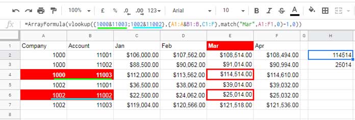
To illustrate, let’s imagine we have a General Ledger (GL) Data sheet for a fictional company. We want to find the value corresponding to the company code “1000” and the account code “11003” in columns A and B respectively (vertical lookup). Additionally, we’ll search for the month “Mar” in row #1 (horizontal lookup).

As we unravel our formula, we’ll eventually uncover the value we seek – $114,514.00, residing in cell E4.
A Non-Array Formula for Three-way Lookup
Now, let’s delve into the non-array formula that works wonders in Google Sheets. This formula may not expand the results to additional rows or columns, but it will do the trick for our purposes.
=ArrayFormula(vlookup(1000&11003,{A1:A&B1:B,C1:F},match("Mar",A1:F1,0)-1,0))You might notice that this formula looks similar to a two-way lookup formula, with a slight tweak in the vertical lookup search keys. We combine the search keys using the ampersand, including the columns A and B.
Decoding the Google Sheets 3-way Lookup Formula
Let’s break down the magic behind our three-way lookup formula and uncover some key points about the Vlookup function in Google Sheets.
By default, VLOOKUP is set to use the search key in the first column of the range. However, we have some flexibility here. In our GL data example, the first search key, “1000,” resides in column A, while the second search key, “11003,” resides in column B.
To handle this, we combine the two search keys using the ampersand, including the columns A and B in the GL data. Therefore, we end up with one search key and one search column, eliminating the need for a second column.
The combined search key: 1000&11003
The combined columns in GL data: {A1:A&B1:B,C1:F}
Now, let’s address the third search key, “Mar,” which corresponds to the month in row #1. Our goal is to return the index column dynamically in Vlookup using the search key.
In this case, the formula match("Mar",A1:F1,0)-1 will return 4 as the result. Although the column that contains the March month data is actually column E (the fifth column), we must deduct 1 due to our combined columns A and B.
And just like that, we have unravelled the easiest formula to execute a three-way lookup in Google Sheets.
Elevating the Game: Array Formula for Three-way Lookup
Now, if you want to take it up a notch and obtain multiple row outputs in a three-way lookup, this is where the array formula comes into play. It builds upon our non-array formula, allowing for more rows.
Here’s the formula you’d use:
=ArrayFormula(vlookup({1000&11003;1002&11002},{A1:A&B1:B,C1:F},match("Mar",A1:F1,0)-1,0))By comparing this formula with the non-array version, you’ll notice that the change lies in the usage of search keys. Take a look at the underlined search keys in cyan and red, not just in the formula bar, but also in columns A and B.
Lastly, I must discuss how to refer to criteria from cells. Here’s the formula in cell J2 as an example:
=ArrayFormula(vlookup(H2:H3&I2:I3,{A1:A&B1:B,C1:F},match(J1,A1:F1,0)-1,0))And there you have it! With these formulas up your sleeve, you can now confidently perform three-way lookups in Google Sheets. I hope you’ve enjoyed this journey into the depths of data exploration.
For more resources on Vlookup and other useful Google Sheets techniques, be sure to visit Crawlan.com. Happy exploring!


