Imagine you’re working on a complex spreadsheet in Google Sheets, and you want to ensure that certain cells are not accidentally edited. Wouldn’t it be great if there was a simple way to lock and unlock cells with just a click? Well, guess what? There is! And it involves the ingenious use of tick marks, also known as checkboxes, in Google Sheets.
Lock and Unlock Cells Using Multiple Checkboxes
Let’s start with a scenario where you want to lock and unlock cells in a specific range using multiple checkboxes. Here’s how you can set it up:
- First, select the cells where you want to insert the checkboxes. In this example, we’ll use cells E2 to E5.
- Go to the Insert menu and click on Tick box to insert the checkboxes.
- Next, select the range of cells that you want to lock and unlock. In this case, we’ll choose cells A2 to D5.
- Navigate to the Data menu and click on Data Validation. Set up the data validation rule as shown in the image below.
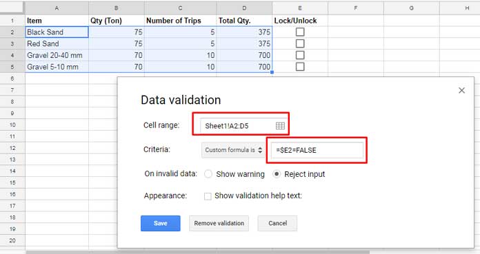
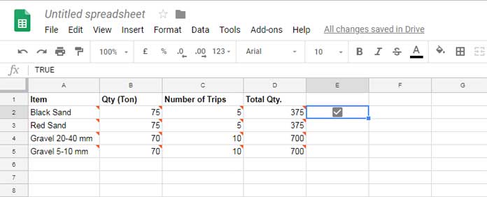
That’s it! Now, when you check a tick box, the corresponding cells in that row will be locked, and you won’t be able to edit their content. To regain editing permission, simply uncheck the tick box. This method allows you to have control over individual rows with ease.
But wait, there’s more!
Lock and Unlock Cells Using One Single Checkbox
If you have a larger range of cells that you want to lock and unlock, you can do so with just one checkbox. Let’s see how:
- Similar to the previous method, select the cell where you want to insert the single checkbox. In this case, we’ll use cell E1.
- Insert the checkbox by going to the Insert menu and clicking on Tick box.
- Again, select the range of cells that you want to lock and unlock, which is A2 to D5 in this example.
- Navigate to the Data menu and go to Data Validation. Set up the data validation rule with the custom formula
=$E$2=FALSE.
And there you have it! With just one tick box, you can now lock and unlock an entire range of cells in Google Sheets. It’s a simple and efficient way to maintain control over your data.
But there’s more to tick marks and checkboxes in Google Sheets than just locking and unlocking cells. Here are some additional tips and tricks that you might find useful:
- How to Convert TRUE/FALSE to Checkboxes in Google Sheets.
- Change the Tick Box Color While Toggling in Google Sheets.
- Assign Values to Tick Box and Total It in Google Sheets.
- 10 Best Tick Box Tips and Tricks in Google Sheets.
Now that you have these valuable insights into using tick marks to your advantage, go ahead and explore the power of checkboxes in Google Sheets. It’s time to take your spreadsheet skills to the next level!
For more helpful tips and tricks, visit Crawlan.com. Happy sheeting!


