Have you ever encountered the challenge of using the same criterion field twice in functions like DSUM, SUMIFS, SUMPRODUCT, or QUERY in Google Sheets? It can be quite tricky, but fear not! In this article, we’ll explore different approaches to tackle this issue and find the most effective method to solve it.
Combine Two SUMIFS Formulas
One approach to using the same criteria field twice in the SUMIFS function is by combining two SUMIFS formulas. Here’s how it works:
=SUMIFS(C7:C,A7:A,"Philip Nida",B7:B,"North")+ SUMIFS(C7:C,A7:A,"Philip Nida",B7:B,"South")By adding two SUMIFS formulas together, each with a different criterion in the same range, you can achieve the desired result. To make it even more convenient, you can replace the hardcoded criteria with cell references:
=SUMIFS(C7:C,A7:A,C1,B7:B,C2)+ SUMIFS(C7:C,A7:A,C1,B7:B,C3)Use a SUBSTITUTE Workaround
Another approach involves using the SUBSTITUTE function to replace one of the criteria with the other. Let’s take a look at an example:
=ArrayFormula(SUMIFS(C7:C14,A7:A14,"Philip Nida",SUBSTITUTE(B7:B14,"South","North"),"North"))In this case, we use the SUBSTITUTE function to replace “South” with “North” in column B. By doing so, we don’t need to use the same criteria field twice in the SUMIFS function. To adapt this formula to cell references, you can use:
=ArrayFormula(SUMIFS(C7:C,A7:A,C1,SUBSTITUTE(B7:B,C3,C2),C2))Use REGEXMATCH
The third approach involves using the REGEXMATCH function to match both criteria in the same range. This function returns TRUE for matching rows, which can be used as the criterion. Here’s an example:
=ArrayFormula(SUMIFS(C7:C14,A7:A14,"Philip Nida",REGEXMATCH(B7:B14, "North|South"),TRUE))To adapt this formula to cell references, you can use:
=ArrayFormula(SUMIFS(C7:C14,A7:A14,C1,REGEXMATCH(B7:B14, C2&"|"&C3),TRUE))Among these three methods, using REGEXMATCH (method #3) is my preferred approach. It allows you to include multiple criteria by simply separating them with a pipe. On the other hand, the SUBSTITUTE method (method #2) requires multiple nesting, and the SUMIFS method (method #1) may clutter the formula with multiple SUMIFS formulas.
In conclusion, the SUMIFS formula does not directly support using the same criteria field more than once without comparison operators. However, by utilizing the SUBSTITUTE function or REGEXMATCH function, we can overcome this limitation and achieve the desired results.
Now that you know these smart workarounds, you can confidently handle the challenge of using the same field twice in the SUMIFS function in Google Sheets. Happy spreadsheeting!
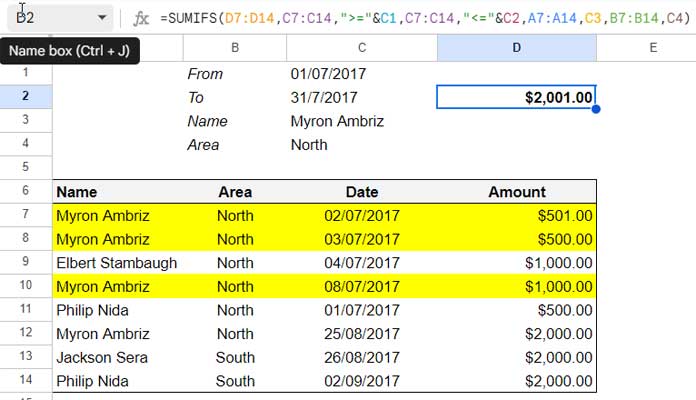
Image source: Crawlan.com


