How to Remove Trailing Zeros from Numbers in Google Sheets

Have you ever encountered the need to remove trailing zeros from numbers in Google Sheets? It can be quite frustrating when these zeros clutter up your data and make it harder to read. But don’t worry, there are simple ways to solve this issue depending on whether the numbers have currency symbols or not.

Removing Trailing Zeros without a Currency Sign

If the number doesn’t contain a currency sign, you can easily remove the trailing zeros by formatting the number back to automatic. Just follow these steps:

1. Select the cell range that contains the numbers.
2. Click on Format > Number > Automatic.

Removing Trailing Zeros from Currency-Formatted Numbers

But what if your numbers are currency-formatted? In this case, you can’t simply use the automatic formatting option as it will remove the currency symbols as well. However, there is still a solution!

You can use a REGEXREPLACE formula in a helper cell to remove the trailing zeros from currency-formatted numbers. Here’s how:

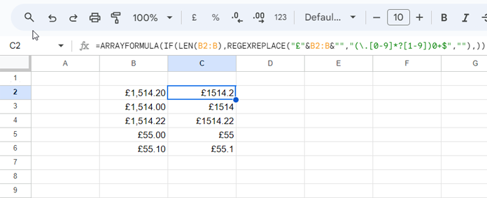
1. Insert the following formula in a blank cell next to your range of currency-formatted numbers:

   =ARRAYFORMULA(IF(LEN(B2:B),REGEXREPLACE("£"&B2:B,"(.[0-9]*?[1-9])0+$",""),))

2. Replace “£” in the formula with the currency symbol used in your range.

Note: If your keyboard doesn’t have your currency symbol, you can use the following formula in any blank cell, copy the result, and paste it into the main formula:

=LEFT(B2)

The result will be in text format. To align it properly, select the converted numbers and right-align them using Format > Alignment > Right.

When using the converted numbers for calculations, make sure to wrap them with the VALUE function. For example:

=ARRAYFORMULA(SUM(VALUE(C2:C6)))

Anatomy of the Formula

Let’s break down the formula we used to remove trailing zeros from currency-formatted numbers:

• ARRAYFORMULA: This function applies the formula to all cells in the specified range and returns an array of results.
• IF(LEN(B2:B),…): It checks if each cell in the range contains a value. If it does, the formula returns the result of the REGEXREPLACE function. Otherwise, it returns an empty string.
• REGEXREPLACE("£"&B2:B,"(.[0-9]*?[1-9])0+$",""): This part of the formula removes all trailing zeros from the number in each cell, after the decimal point.

That’s it! Now you know how to remove trailing zeros from numbers in Google Sheets, whether they have currency symbols or not. It’s time to clean up your data and make it more readable. If you want to dive deeper into Google Sheets features, don’t forget to check out Crawland.com for more helpful tips and tricks.